
Spectral profiler#
The Spectral Profiler Widget allows you to view region spectra from image cubes. There are two modes:
single-profile mode (when none of the “Image”/”Region”/”Statistic”/”Polarization” checkboxes is selected)
multiple-profile mode (when one of the “Image”/”Region”/”Statistic”/”Polarization” checkboxes is selected)
The single-profile mode allows you to create multiple Spectral Profiler Widgets and compare spectra side by side. The multiple-profile mode, however, shows multiple spectra in one plot with the same x and y ranges so that spectra can be compared directly.
Note
Rendering performance
When displaying a spectral profile with the number of channels more than the number of screen pixels of the Spectral Profiler Widget, a decimated profile will be derived and displayed to you as an enhancement of performance. Min/max decimation of a profile is adopted to ensure profile features are preserved. In other words, positive and negative peaks should stay at the same screen pixels, just like displaying the full-resolution profile. Decimation with narrower and narrower intervals is applied when you keep zooming in the profile. A full-resolution profile is displayed when the number of screen pixels is more than the number of pixels of the profile to be displayed.
Single-profile mode#
The four dropdown menus and their selection states determine how spectral profiles are extracted from image cubes and displayed. When there is no checkbox selected, the Spectral Profiler Widget displays one spectrum only depending on the selection of each dropdown menu (”Image”, “Region”, “Statistic”, and “Polarization”).
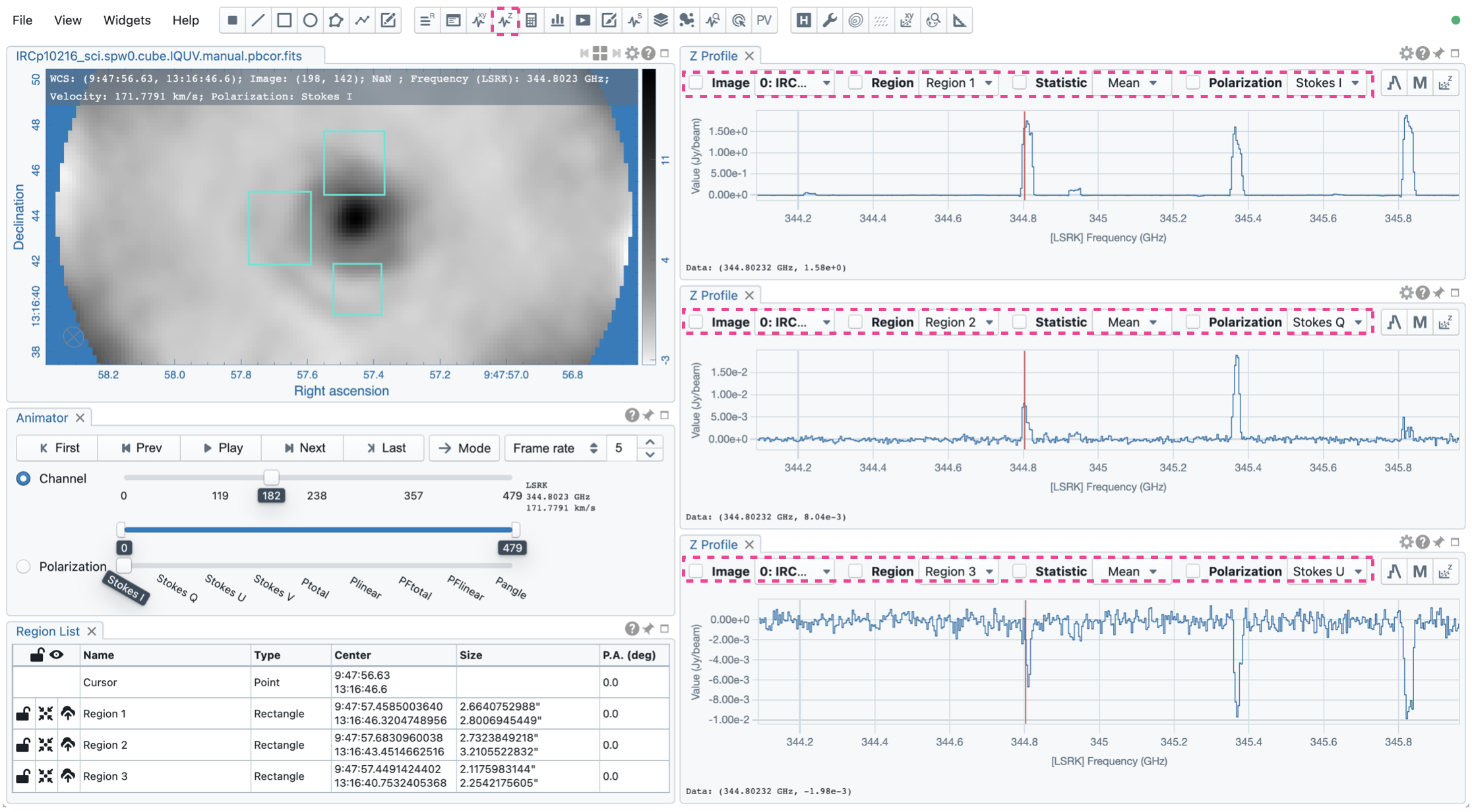
When regions are created, the Spectral Profiler Widget can be configured to display a profile from a specific region with the “Region” dropdown menu. The default of the “Region” dropdown menu is “Active”, which points to the active (selected) region. If no region is active, it defaults to the cursor region. The “F” key will turn the cursor profile live update on or off. When cursor update is disabled, a marker “+” will be placed on the image to indicate the position of the profile taken.
Additional statistic types to compute the region spectral profile are available with the “Statistic” dropdown menu (default to mean). If the image cube has multiple polarization components, the “Polarization” dropdown menu will be activated and defaulted to “Current”, which is synchronized with the selection in the Animator. Select the “Polarization” dropdown menu to view a specific polarization component.
Multiple Spectral Profiler Widgets can be configured to display different region (”Region” dropdown menu) spectral profiles from different image cubes (”Image” dropdown menu) and polarization (”Polarization” dropdown menu, if applicable) with different statistics (”Statistic” dropdown menu), allowing a side-by-side comparison of spectra.
Multiple-profile mode#
When one of the “Image”, “Region”, “Statistic”, and “Polarization” checkboxes is selected, the Spectral Profiler Widget switches to the multiple-profile mode. CARTA supports four different use cases as the following:
Comparing spectra from different image cubes:
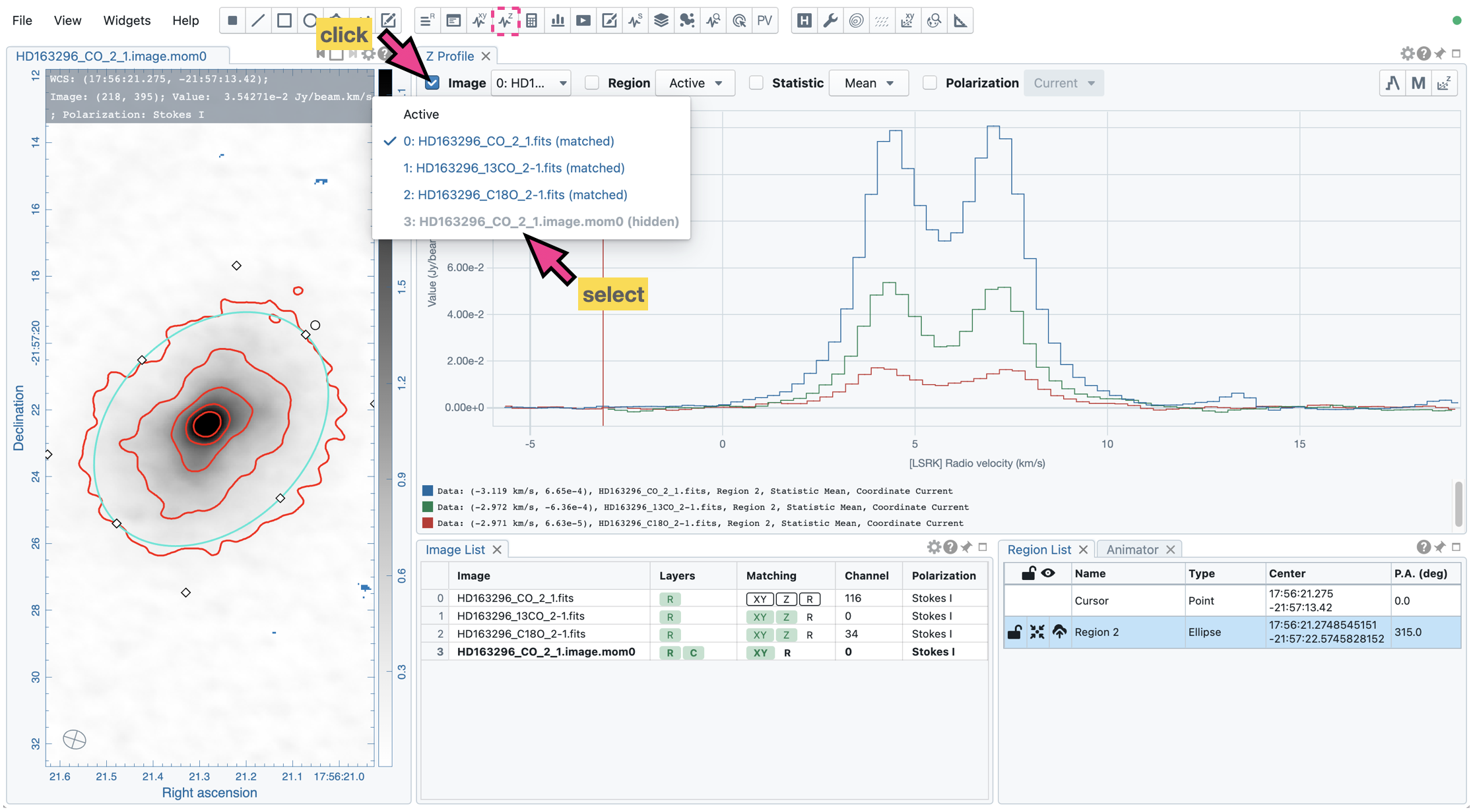
When the “Image” checkbox is selected, spectral profiles from different spatially and spectrally matched cubes can be displayed. The “Image” dropdown menu shows the matching state of each image as configured via the Image List Widget. The dropdown menu allows single-selection only. The selected image and its matched images are used for spectral profile computations based on the selected region (single selection), statistic (single selection), and polarization (if applicable, single selection). In the following example, CO 2-1, 13CO 2-1, and C18O 2-1 lines from the source HD163296 are plotted for comparison. The profiles are derived from the rectangle region with mean statistics.
Comparing spectra from different regions:
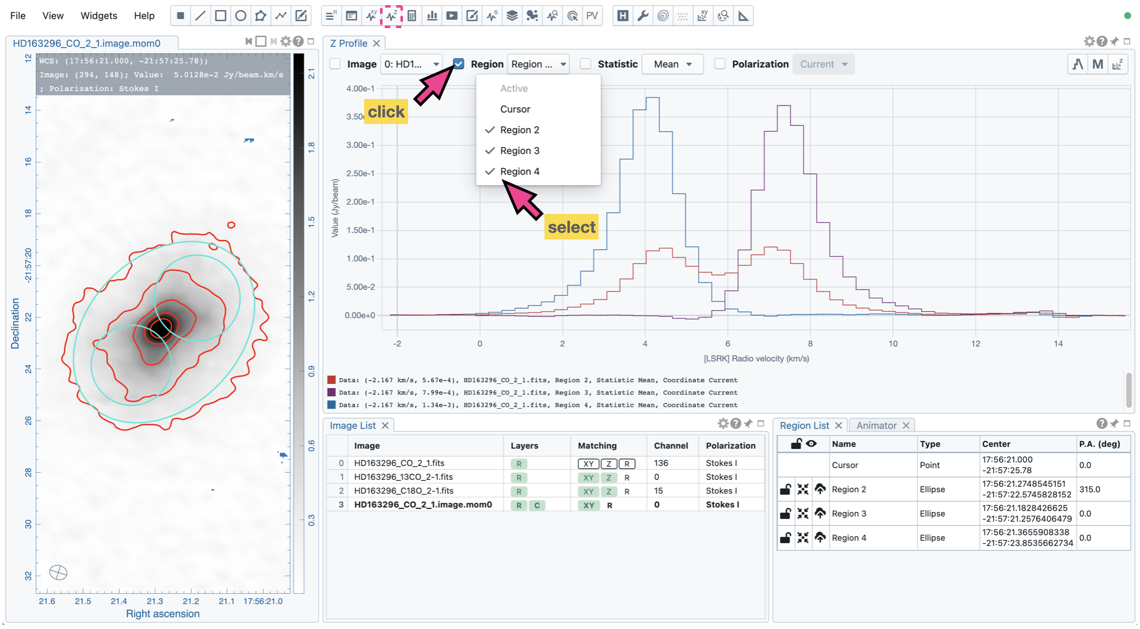
When the “Region”” checkbox is selected, spectral profiles from different regions of an image cube can be displayed. The “Region” dropdown menu allows multiple selections of different regions. The region spectral profiles will be computed based on the selected image (single selection), statistic (single selection), and polarization (if applicable, single selection). The following example compares CO 2-1 mean spectra from different parts of the protoplanetary disk HD163296.
Comparing spectra with different statistical quantities:
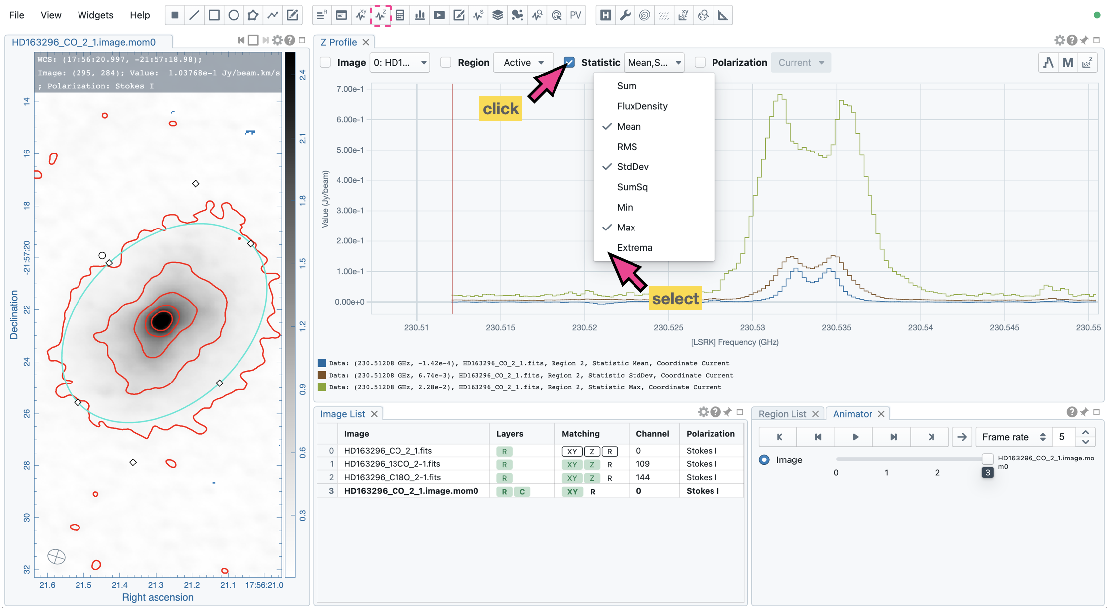
When selecting the “Statistic” checkbox, region spectral profiles with different statistical quantities can be displayed. The “Statistic” dropdown menu allows multiple selections of different statistical quantities. The region spectral profiles will be computed based on the selected image (single selection), region (single selection), and polarization (if applicable, single selection). In the following example, CO 2-1 mean, standard deviation, and max spectra are compared. The profiles are derived from the ellipse region.
Comparing spectra with different polarization components:
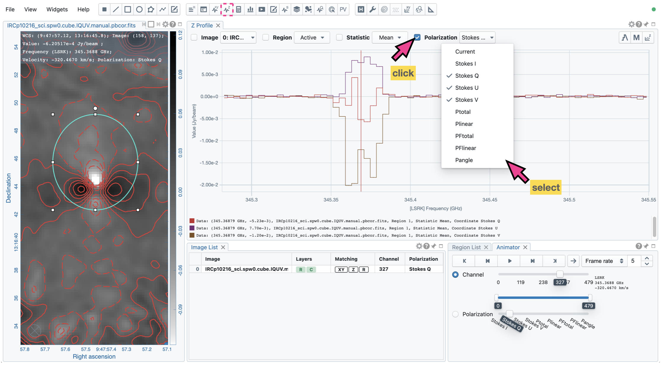
When the “Polarization” checkbox is selected, region spectral profiles with different polarization components can be displayed. The “Polarization” dropdown menu allows multiple selections of polarization components, including computed components. The region spectral profiles will be computed based on the selected image (single selection), region (single selection), and statistic (single selection). The following example compares Stokes Q, U, and V region spectra from IRC+10216.
Note
Only one of the “Image”, “Region”, “Statistic”, and “Polarization” checkboxes can be selected at a time. For example, plotting spectral profiles from different images and multiple regions in the same plot is prohibited.
Interactivity#
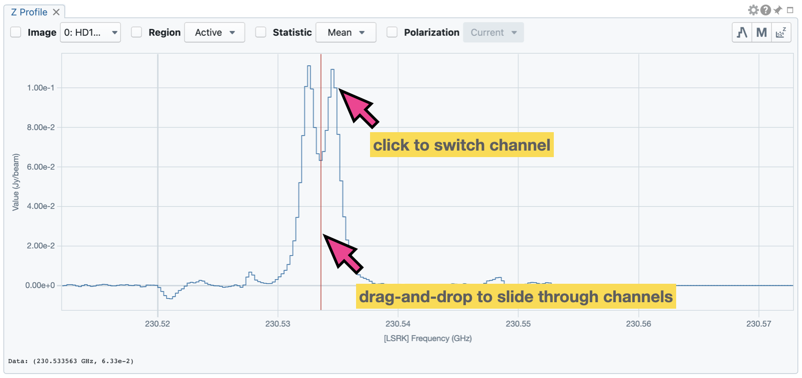
The interactions of the Spectral Profiler Widget are demonstrated in the section Chart interactions. The red vertical bar indicates the channel of the image displayed in the Image Viewer. Clicking directly on the spectral profile plot will change the displayed image to the clicked channel. Alternatively, the red vertical bar is draggable and acts just like the channel slider of the Animator Widget.
Spectral convention and intensity unit#
The x axis shows the spectral coordinate and the y axis shows the pixel values. Additional options to configure the profile plot are available in the Spectral Profile Settings Dialog, which can be launched by clicking the “cog” button in the top-right corner. In the dialog, you may select a different spectral convention (e.g., optical velocity), a different reference system (e.g., TOPO), and a different intensity unit (e.g., K) with the “Conversion” tab. You can enable the display of a secondary spectral value at the bottom of the Spectral Profiler Widget.
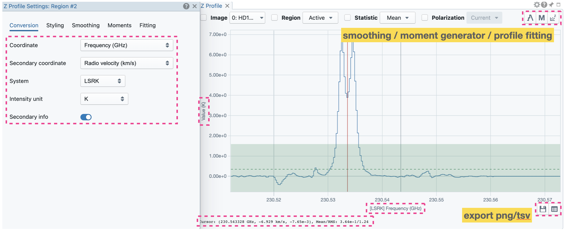
The spectral convention with equivalent units includes the following options:
Frequency
Radio velocity
Optical velocity
Vacuum wavelength
Air wavelength
Squared air wavelength
Squared vacuum wavelength
Channel
The reference system includes the following options:
LSRK (Local Standard of Rest, Kinematic)
LSRD (Local Standard of Rest, Dynamical)
Barycentric
Topocentric
Profile smoothing#
The displayed profile can be smoothed via the options in the “Smoothing” tab (see section Profile smoothing) of the Spectral Profile Settings Dialog. A shortcut button to access this tab is available in the top-right corner of the Spectral Profiler Widget.

Moment map genertator#
Image collapsing is available in the “Moments” tab (see section Moment image generator) of the Spectral Profile Settings Dialog. A shortcut button to access this tab is available in the top-right corner of the Spectral Profiler Widget.

Profile fitting#
Profile fitting is available in the “Fitting” tab (see section Profile fitting) of the Spectral Profile Settings Dialog. A shortcut button to access this tab is available in the top-right corner of the Spectral Profiler Widget.

Custom rest frequency#
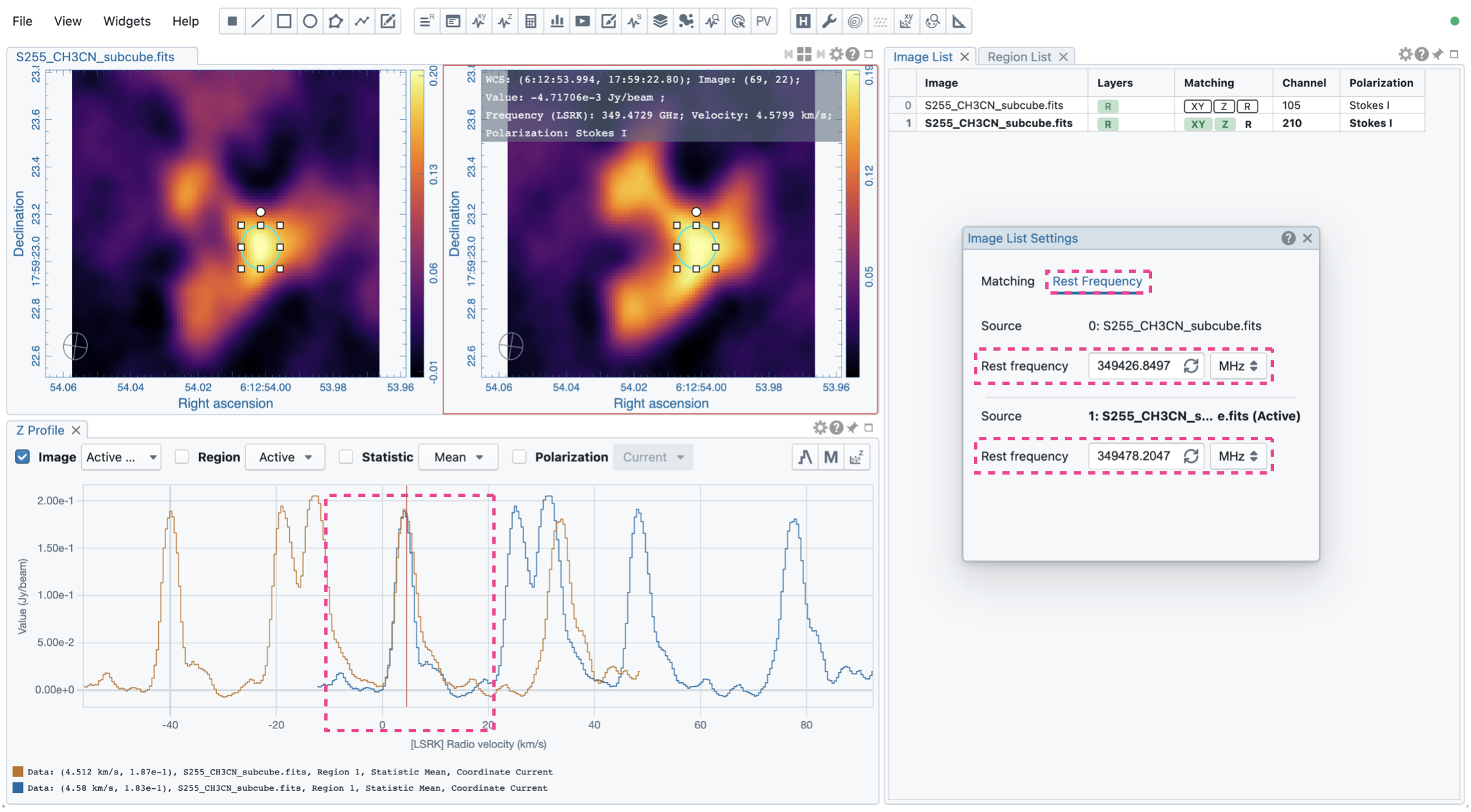
A custom reference rest frequency can be applied to an image cube to temporarily overwrite the RESTFRQ header with the settings dialog of the Image List Widget. The velocity axis will be recomputed once a custom rest frequency is given. This feature allows you to compare different spectral line profiles in the velocity domain efficiently without changing the RESTFRQ header repeatedly and permanently. Note that with the “File” -> “Save image” dialog, you can set a new rest frequency to the saved image (i.e., overwriting the RESTFRQ header).
In the following example, a cube containing five major spectral lines is loaded twice in CARTA. Two custom rest frequencies are applied to the cubes, respectively. We can directly compare the two target profiles in the velocity domain with the multiple-profile plotting mode, as their velocities have been recomputed based on the custom rest frequencies instead of the RESTFRQ header. As the velocity axis of each cube is recomputed, spectral matching in the velocity domain is re-applied automatically. Images from the two target lines can be compared directly near the systemic velocity of the source.
Styling#
The Styling tab in the Spectral Profiler Settings Dialog allows you to configure the profile plot style.

The option “Show mean/RMS” in the “Styling” tab will use the data in the current view to derive a mean value and an RMS value and visualize the results on the plot. Numerical values are also displayed in the bottom-left corner of the Spectral Profiler Widget. When the cursor is on the image in the Image Viewer, the pointed pixel value (frequency, velocity, or channel index, and pixel value) will be displayed in the bottom-left corner of the Spectral Profiler Widget. When the cursor is on the spectral profile plot, the pointed profile data will be displayed instead.
Export#
The profile can be exported as a PNG image or a text file in TSV format via the toolbar at the bottom-right corner of the Spectral Profiler Widget.
Settings#
The Spectral Profiler Settings Dialog provides options to configure the Spectral Profiler Widget including:
Conversion: to configure the spectral convention, reference system, and intensity unit (see Spectral convention and intensity unit)
Styling: to configure the profile plot style
and tools associated with spectral cube analysis, including:
Profile smoothing: to configure the profile smoothing (see Profile smoothing)
Moment map generation: to configure the moment map generation (see Moment image generator)
Profile fitting: to configure the profile fitting (see Profile fitting)