Spatial profiler#
The Spatial Profiler provides computed spatial profiles at the cursor position or the point region along a horizontal or vertical cut. It can also compute spatial profiles along a line region or a polyline region.
Note
Rendering performance
When displaying a spatial profile with the number of pixels more than the number of screen pixels of the Spatial Profiler Widget, a decimated profile will be derived and displayed as an enhancement of performance. Min/max decimation of a profile is adopted to ensure profile features are preserved. In other words, positive and negative peaks should stay at the same screen pixels, just like displaying the full-resolution profile. Decimation with narrower and narrower intervals is applied when you keep zooming in the profile. A full-resolution profile is displayed when the number of screen pixels is more than the number of pixels of the profile to be displayed.
Note
Profile fitting capability will be added in a future release.
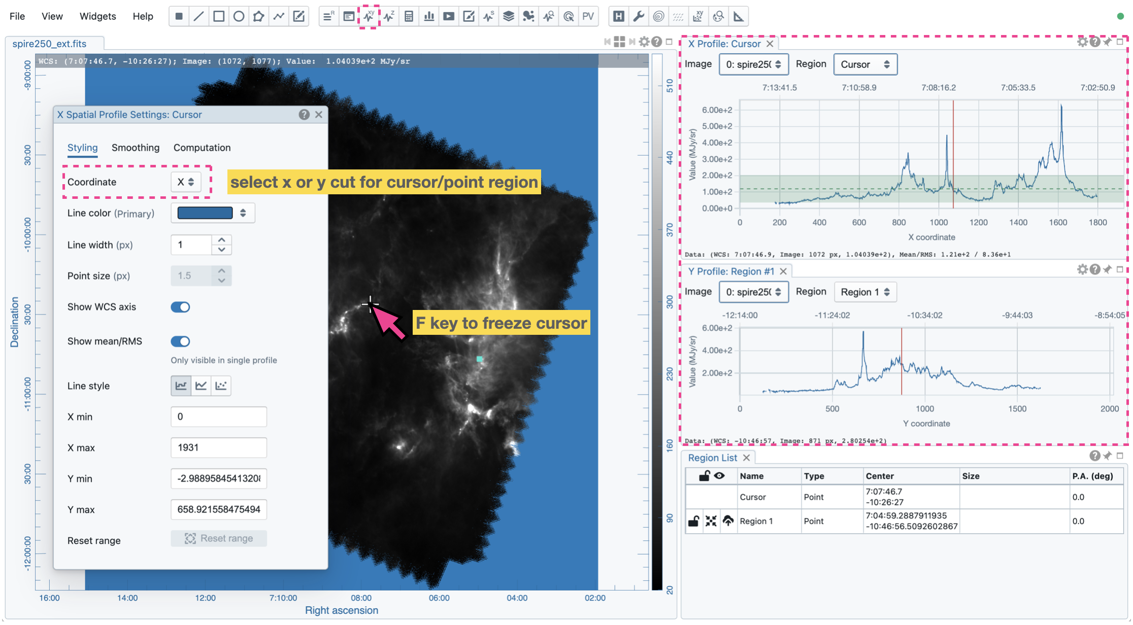
Cursor region or point region#
When the “Region” dropdown menu is set to “cursor”, or a point region, a horizontal or a vertical profile is extracted from the “Image” depending on the selection in the Spatial Profiler Settings Dialog (the “cog button at the top right corner”). When the cursor moves on the image, profiles derived from the full-resolution raster image are displayed. The “F” key will turn the profile live update on or off. When cursor update is disabled, a marker “+” will be placed on the image to indicate the position of the profiles taken.
Line region or polyline region#
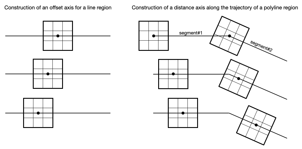
When a spatial profile is derived from a line or a polyline region, a set of boxes with a “height” (parallel to the trajectory) of three unit steps and a custom “width” (perpendicular to the trajectory; set with the “Computation” tab of the Spatial Profiler Settings Dialog) in number of unit steps are created along the trajectory. These hidden boxes are created on the reference image first. Then, similar to the polygon approximation of closed regions, these “boxes” are transformed into the spatially matched secondary image to derive a spatial profile.
If the image is considered “flat” without noticeable distortion, the unit step refers to an image pixel. However, if the image is considered “wide” with noticeable distortion, the unit step refers to the angular size of an image pixel as defined in the image header. In this case, the boxes retain approximately a fixed solid angle. All these approximations allow spatial profiles of the same trajectory among different spatially matched images to be compared directly.
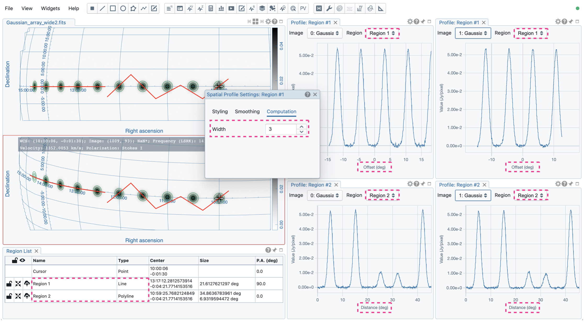
An “offset” axis is constructed to compute a spatial profile for a line region. The origin is the middle point of the line region. A “distance” axis is constructed for a polyline region to compute a spatial profile along the trajectory. The origin is the first control point of the polyline. Note that sampling artifacts may be seen near the endpoints of a line region or each control point of a polyline due to the rounding effect of the sampling process.
Note
When the sampling process is made along a line region or a polyline region in a “non-flat” image, the solid angle of the sampling boxes is approximately conserved. In some cases, especially when the image is highly distorted, some computed boxes may cover no image pixel for profile calculations. Therefore, you may see NaN values in the final spatial profile. When this happens, you can consider increasing the averaging “width” with the “Computation” tab of the Spatial Profiler Settings Dialog.
In a future release, the averaging “height” (parallel to the trajectory) can be customized too. With the v6.0 release, the “height” is fixed to three (three pixels for flat image or three unit angular size for non-flat image).
Interactivity#
The interactions of the Spatial Profiler Widget are demonstrated in the section Chart interactions. The red vertical bar indicates the pixel where the cursor profile is taken. The bottom axis shows the image coordinate for the cursor or point region, offset coordinate for the line region, and distance for the polyline region. An optional world coordinate is displayed on the top axis for cursor or point region.
The option “Show mean/RMS” in the “Styling” tab will use the data in the current view to derive a mean value and an RMS value and visualize the results as a green shaded area on the plot. Numerical values are also displayed at the bottom-left corner. When the cursor is on the image in the Image Viewer, the pointed pixel value (pixel index and pixel value) will be displayed at the bottom-left corner of the Spatial Profiler. When the cursor is on the Spatial Profiler graph, the pointed profile data will be displayed instead.
Profile smoothing#
The displayed profile can be smoothed with different methods in the “Smoothing” tab (see section Profile smoothing).

Styling#
The profile plot can be styled with the “Styling” tab of the Spatial Profiler Settings Dialog.

Export#
The profile can be exported as a PNG image or a text file in TSV format via the toolbar at the bottom-right corner when you hover over the plot.
Settings#
The Spatial Profiler Settings Dialog contains the following tabs:
Computation: set the averaging width for the line or polyline region (see Line region or polyline region).
Smoothing: set the smoothing method and parameters for the profile (see Profile smoothing).
Styling: set the styling of the profile plot (see Styling).