
Fundamental ideas#
GPU-accelerated client-side rendering#
CARTA utilizes an efficient approach, “tiled rendering”, to display a raster image. In the Image Viewer, you see an ensemble of image tiles (default 256 pixels by 256 pixels) processed in parallel.
As shown in the figure below, if we have an image with 2048 pixels by 2048 pixels, tiles will be constructed in four layers with different downsample factors. The zeroth layer contains only one tile with a size of 256 pixels by 256 pixels. A downsample factor of 8 is applied to the original image to create this tile. The first layer contains four tiles, each with a size of 256 pixels by 256 pixels. The downsample factor of 4 is applied to the original image to create these four tiles. This process continues until no downsampling is required. In this case, the tiles of the third layer are not downsampled.
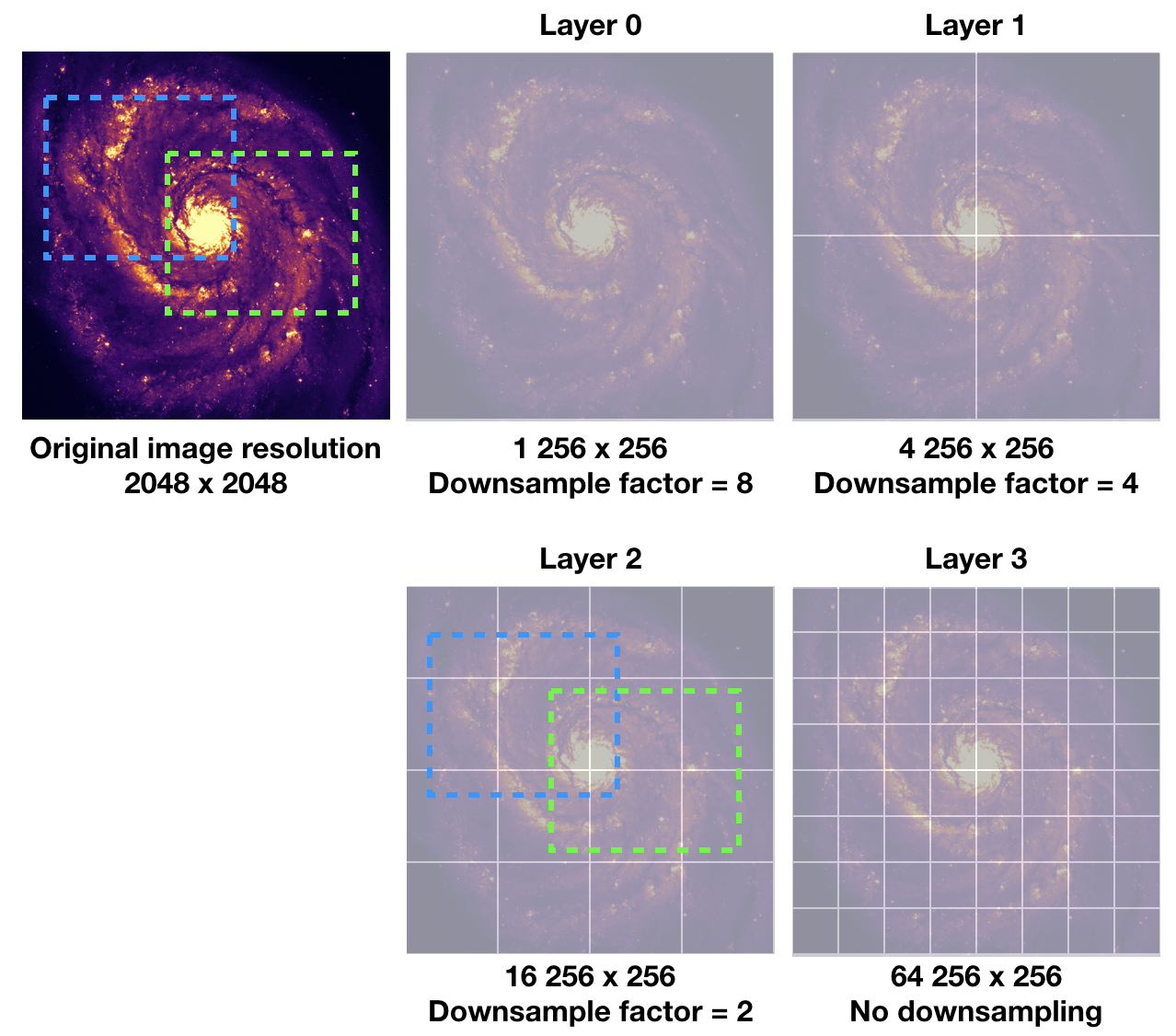
When you change the field of view or the size of the Image Viewer, tile data from the layer matching your screen resolution within a factor of two will be used. For example, if you are interested in the field of the blue box and the Image Viewer has a screen size of 512 pixels by 384 pixels, tiles from the 2nd layer will be used for rendering. In this case, nine tiles will be used. If you pan a little bit around the blue box, no new tile data are required. However, if you pan the view to the green box with the same viewer size, two additional tiles from the second layer are required, and four tiles will be re-used for rendering. With this tiled rendering approach, tiles will be re-used at different zoom levels and with different fields of view to minimize the amount of data transfer while keeping the image sharp on the screen. Effectively, you will see that the image becomes sharper and sharper at higher and higher zoom levels.
The performance of the tiled rendering can be customized with the Preferences Dialog, “File” -> “Preferences” -> “Performance”. The default values are chosen to ensure that raster images are displayed efficiently with sufficient accuracy. Advanced users may refine the setup if necessary. For example, when accessing a remote backend under poor internet conditions, the compression quality might be slightly lowered to make the tile data smaller. Note that a lower compression quality might introduce noticeable artifacts on the raster image. Please adjust with caution.
Alternatively, you may enable the low bandwidth mode, which will reduce required image resolutions by a factor of two (so that the image will look slightly blurry) and cursor responsiveness from 200 ms to 400 ms (HDF5 images: from 100 ms to 400 ms). Under good internet conditions, you may enable streaming image tiles while zooming to see progressive updates of image resolutions at different zoom levels.
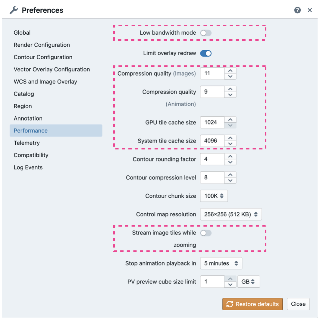
Image matching#
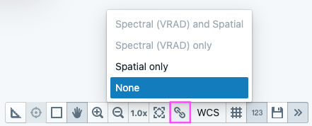
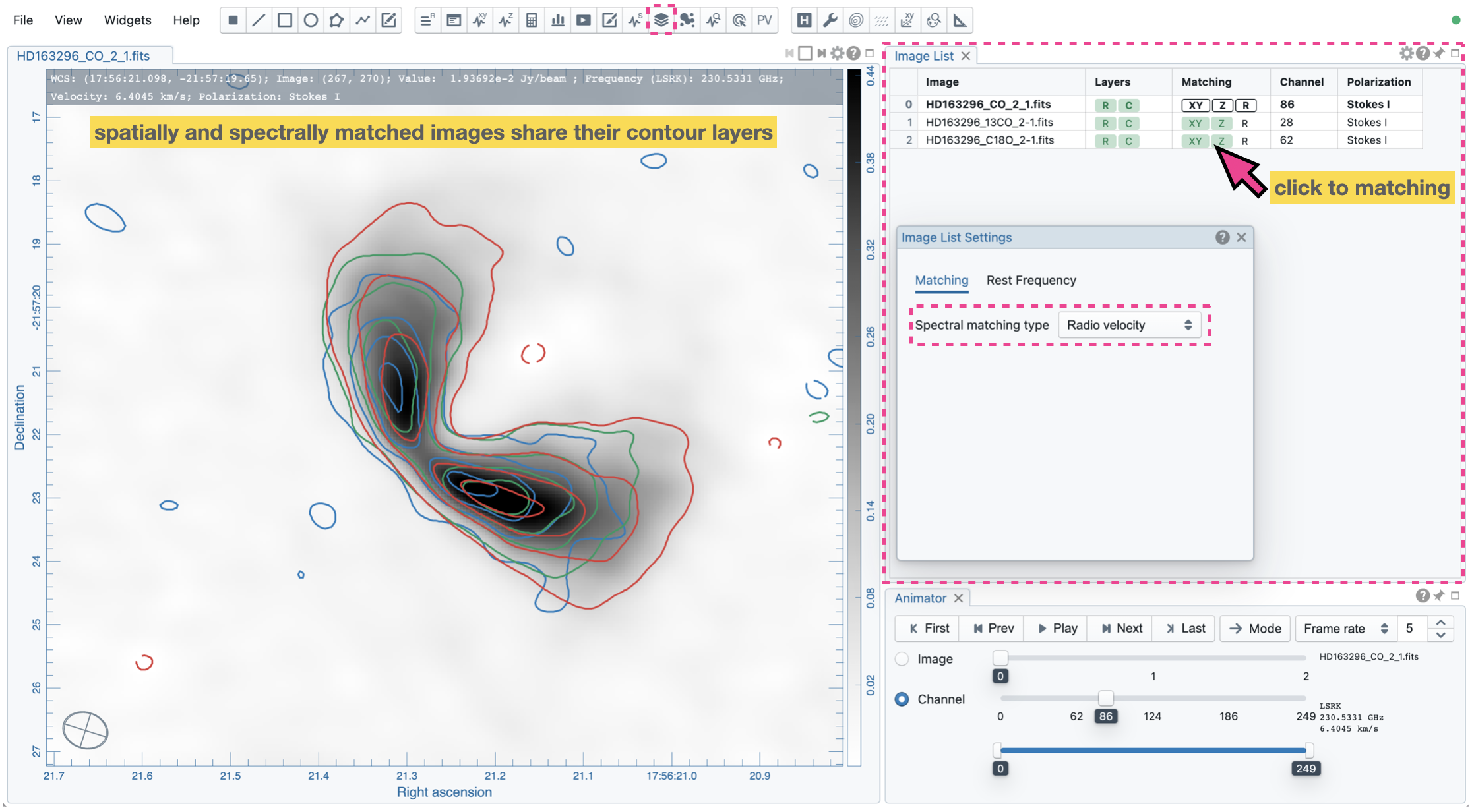
You may trigger image matching based on their world coordinates when multiple images are loaded in CARTA. It is a common practice to compare images from different telescopes or even from the same telescope with different spectral and spatial setups. You can use the “Matching” column of the Image List Widget to trigger the image-matching process,
or the tool button in the Image Viewer.
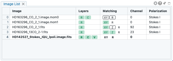
The Image List Widget shows a list of all loaded images, including their:
file name (active image is in boldface)
rendering type (“Layers” column): “R” means raster, “C” means contour, and “V” means vector overlay
image matching state (“Matching” column):
“XY” means the spatial domain. “Boxed” XY means the spatial reference.
“Z” means the spectral domain, “Boxed” Z means the spectral reference.
“R” means the raster rendering configuration. “Boxed” R means the raster rendering reference.
channel index
polarization component
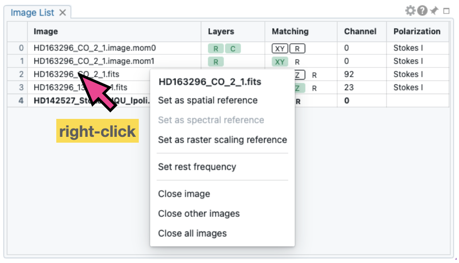
The first loaded image with valid spatial world coordinates serves as the default spatial reference and is highlighted with an open black box (e.g., HD163296_CO_2_1.image.mom0 in the above example). Similarly, the first loaded image with valid spectral coordinates serves as the default spectral reference and is highlighted with an open black box (e.g., HD163296_CO_2_1.fits in the above example). To match the world coordinates of other loaded images, you can click the “XY” button to match the spatial domain and click the “Z” button to match the spectral domain. If you would like to apply the same rendering configuration for different raster images, click the “R” button so that matched images will be rendered in the same way as the reference image highlighted with an open black box (e.g., HD163296_CO_2_1.image.mom0 in the above example).
The “boxed” XY, Z, or R button indicates the reference image for spatial matching, spectral matching, or raster rendering configuration, respectively. Users can click the “boxed” button to trigger the matching process for all applicable images. For example, if you click the “boxed” XY button of the spatial reference image, all other images with valid and matchable spatial world coordinates will be matched in the spatial domain to the reference image. If you click the “boxed” Z button of the spectral reference image, all other images with valid and matchable spectral coordinates will be matched in the spectral domain to the reference image. If you click the “boxed” R button of the raster rendering reference image, all other raster images will be rendered in the same way as the reference image.
You may change a spatial reference image, a spectral reference image, or a raster scaling reference by right-clicking on an image in the Image List Widget and using the context menu.
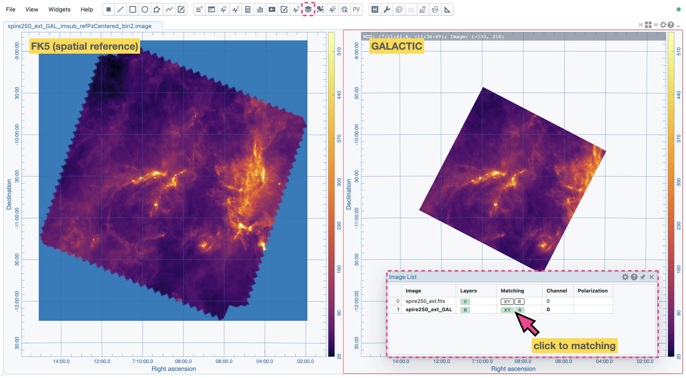
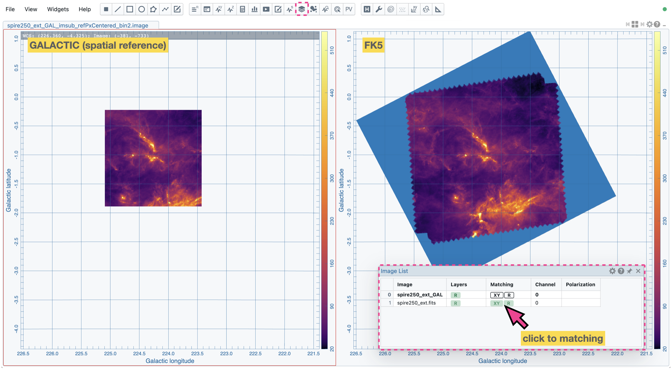
For raster images, matching in the spatial domain is achieved by applying translation, rotation, and scaling to images with respect to the reference image. This is also known as the “affine transformation”.
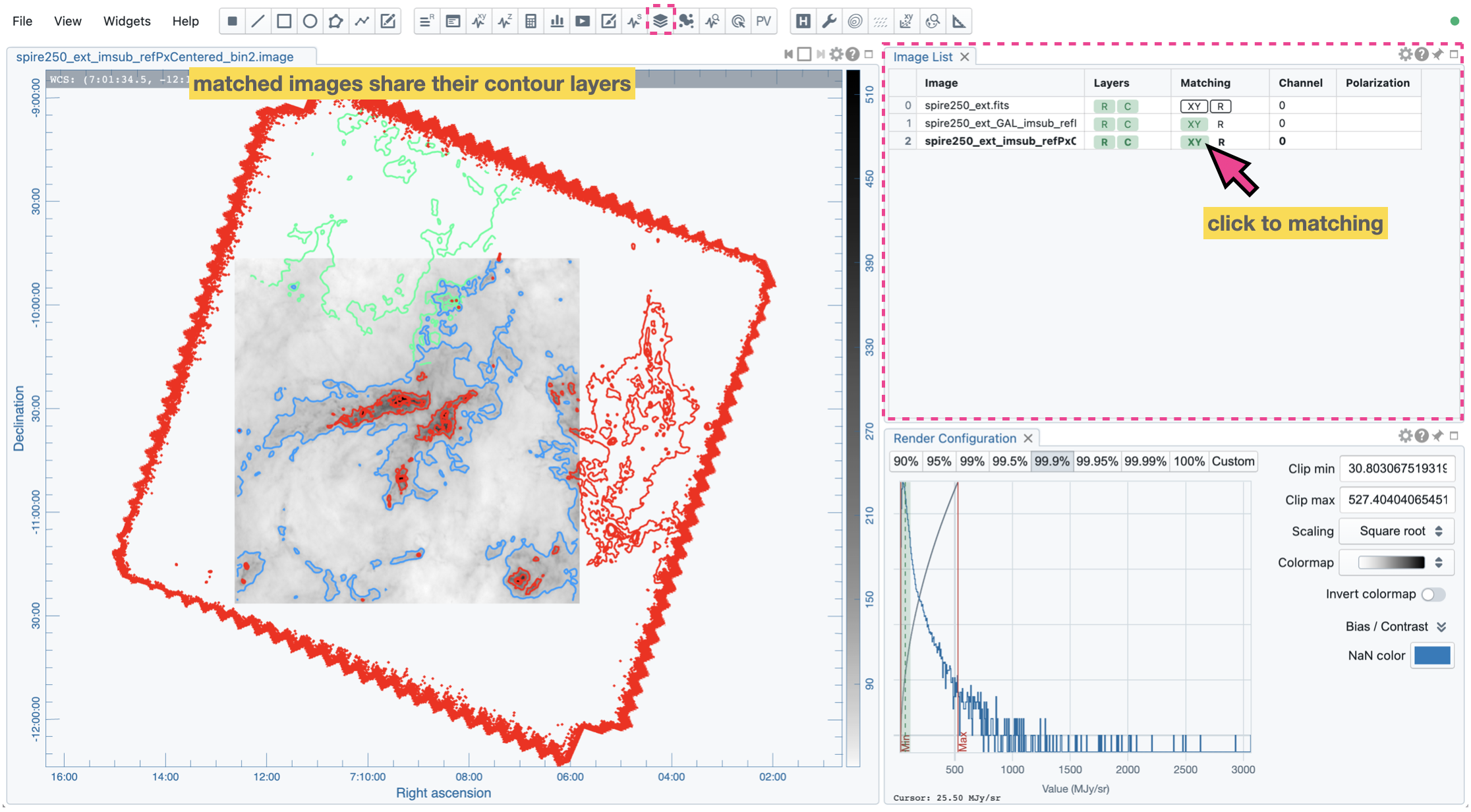
For contour images, matching in the spatial domain is achieved by reprojecting contour vertices to the raster image in the view. Multiple contour images can be displayed on top of a raster image if spatial matching of the target contour image is enabled.
For image cubes, matching in the spectral domain is achieved by nearest interpolation with the target spectral convention. The default is “radio velocity”. The reference convention of spectral matching is configurable with the settings dialog of the Image List Widget. When spectral matching is enabled by clicking the “Z” button, the matched channel indices are updated in the Image List Widget. Images in the Image Viewer Widget are then updated accordingly.
Note
Projection effects of raster images
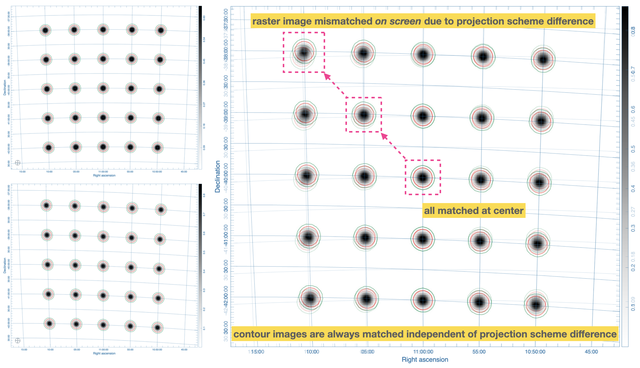
As raster images are matched spatially by applying translation, rotation, and scaling (affine transformation), the projection effects between different images might be visible if images have a wide field of view and/or have very different projection schemes. In the following example, projection effects in raster images are demonstrated. However, the projection effects of contour images are properly handled in CARTA. Contours are reprojected with sufficient accuracy to the raster image, as seen in the Image Viewer.
Note
If a spatial reference image or a spectral reference image is closed via the menu “File” -> “Close image”, all matched images will be unmatched, and a new reference image will be automatically registered.
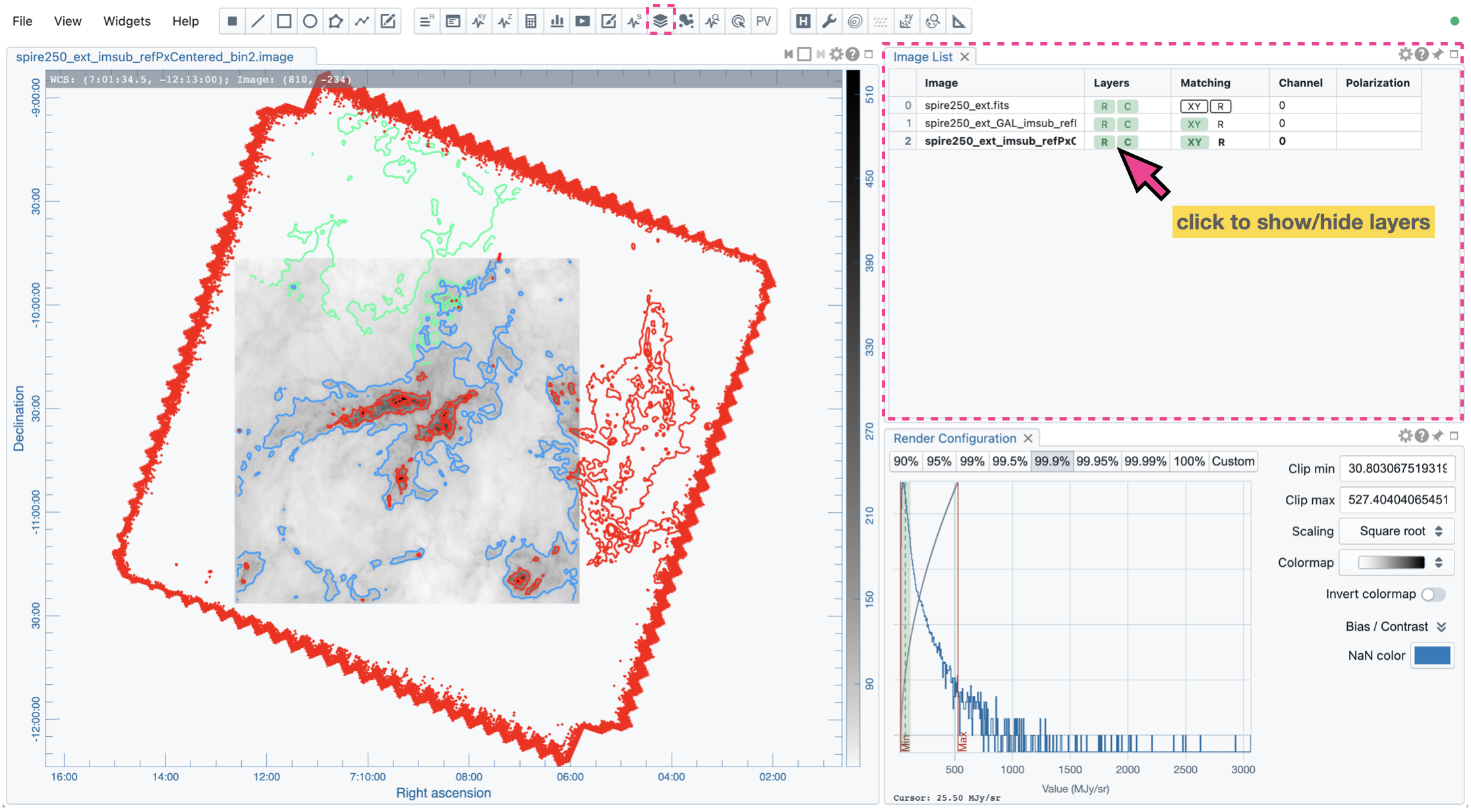
A raster image, contour image, or vector overlay image may be hidden in the Image Viewer by clicking the “R” button, the “C” button, or the “V” button of the “Layers” column in the Image List Widget, respectively. For example, you can create an image with contours only by clicking the “R” button to hide the raster image.
Region of interest#
As of v6.0, CARTA supports the following region types:
rectangle (rotatable)
ellipse (rotatable)
square (rotatable; as a special case of rectangle; “shift” key + drag)
circle (as a special case of ellipse; “shift” key + drag)
point
polygon
line (rotatable)
polyline
The creation and modification of regions are demonstrated in the section Region of interest or image annotation object interactions. To create a region, use the region button from the toolbar at the bottom-right corner of the Image Viewer or use the region buttons from the region bar at the top of the GUI, then use the cursor drag-and-drop action to draw a region. CARTA allows regions to be created even if the region is outside the image. Keyboard controls associated with regions are listed below.
macOS |
Linux |
|
|---|---|---|
Region properties |
double-click |
double-click |
Delete selected region(s) |
del / backspace |
del / backspace |
Toggle region creation mode |
C |
C |
Deselect region(s) |
esc |
esc |
Cancel region creation |
esc |
esc |
Switch region creation mode |
command + drag |
ctrl + drag |
Symmetric region creation |
shift + drag |
shift + drag |
Toggle current region lock |
L |
L |
Unlock all regions |
shift + L |
shift + L |
Pan image (inside region) |
command + click / middle-click |
ctrl + click / middle-click |
Move region (default step) |
arrow keys |
arrow keys |
Move region (coarse step) |
shift + arrow keys |
shift + arrow keys |
Move region (fine step) |
option + arrow keys |
alt + arrow keys |
Copy and paste region |
command + C / command + V |
ctrl + C / ctrl + V |
Multi-select regions |
command / ctrl + click |
ctrl + click |
Multi-select regions |
shift + click-and-drag |
shift + click-and-drag |
Toggle control point editing |
enter |
enter |
Deselect control point |
esc |
esc |
Cycle through control points |
tab or shift + tab |
tab or shift + tab |
Modify control point |
arrow keys |
arrow keys |
Modify control point (coarse) |
shift + arrow keys |
shift + arrow keys |
Modify control point (fine) |
option + arrow keys |
alt + arrow keys |
Tip
“backspace” does not delete a region…
If using CARTA remote mode in Firefox on macOS, you may find the “backspace” key navigates back a page instead of removing a region. This behavior can be prevented by modifying your Firefox web browser settings:
Enter about:config in the address bar.
Click “I accept the risk!”
A search bar appears at the top of a long list of preferences. Search for “browser.backspace_action”
It will likely have a value of 0. Double-click it, and then modify it to a value of “2”.
Close the about:config tab, and now backspace will no longer navigate back a page.
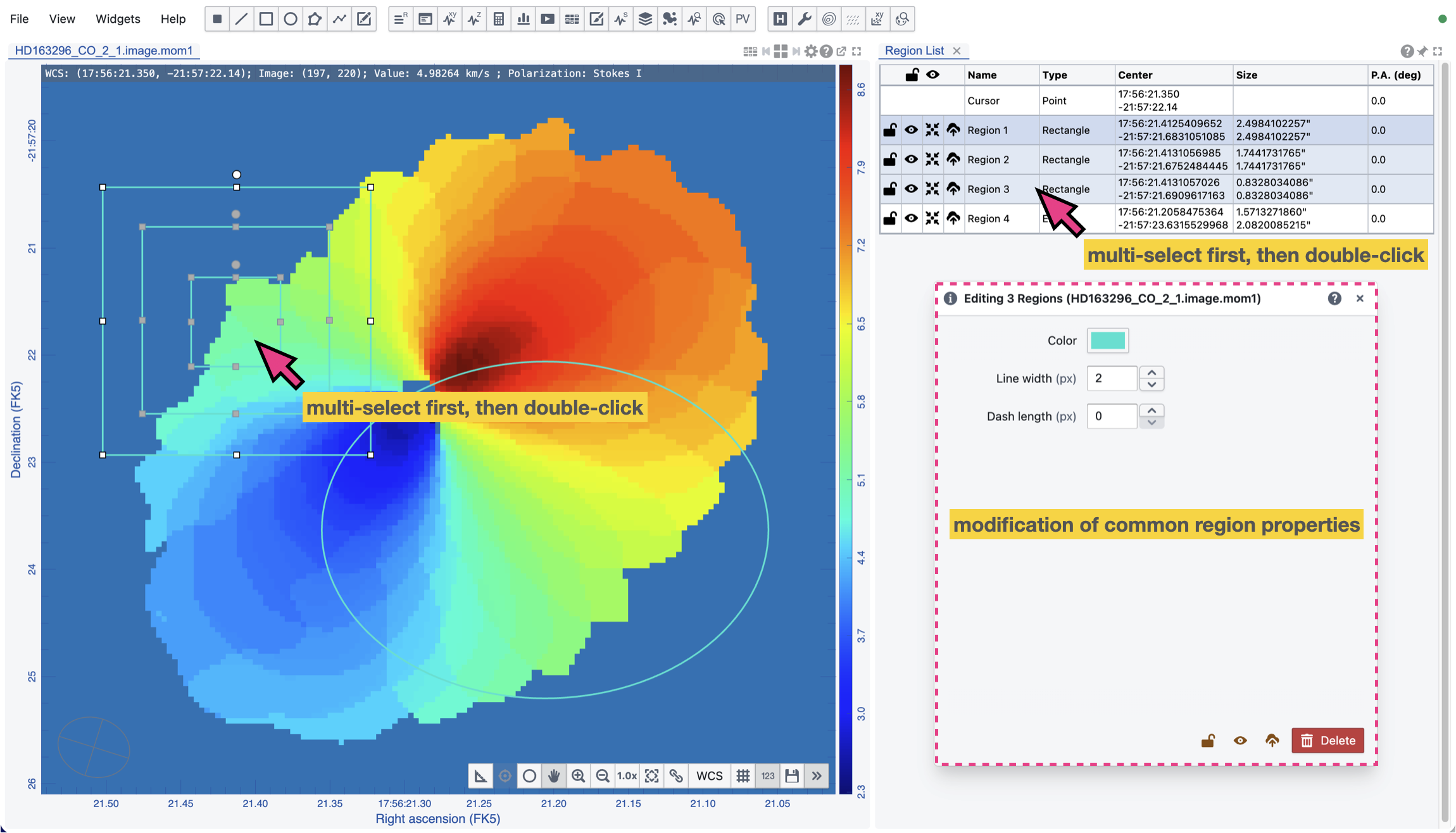
All created regions are listed in the Region List Widget with basic region properties. To select a region (region state changes to “active”), click on the region in the Image Viewer or the region in the Region List Widget. To multi-select regions, use the “shift” key and click on the regions in the Image Viewer or the Region List Widget. You can also multi-select regions by holding the “shift” key and clicking and dragging a box to enclose the regions in the Image Viewer. Alternatively, you can use the “command” key / “shift” key on macOS, or the “ctrl” key / “shift” key on Linux as the modifier key to multi-select regions by clicking the regions in the Region List Widget. When multiple regions are selected, you can modify their common properties simultaneously with the Region Configuration Dialog.
To modify the properties of a selected region, double-click on a region in the Image Viewer or a region in the Region List Widget to bring up the Region Configuration Dialog. A region’s color, line style, name, location, and shape are all configurable with the Region Configuration Dialog. The location and shape properties can be edited in the image coordinates or in the world coordinates with angular scales (default). When mutiple regions are selected, only the common properties among the selected regions are shown in the Region Configuration Dialog.
To de-select a region or a set of regions, or cancel a region creation process, press the “esc” key. Press the “delete” or “backspace” key to delete a selected region or selected regions.
An active region can be locked by pressing the “L” key or clicking the “lock” button in the Region List Widget or region property dialog. You may lock all regions at once by clicking the “lock” button in the top-left corner of the Image List Widget. When a region is locked, it cannot be modified (resize, move, or delete) with mouse actions and the “delete” or “backspace” key. A locked region, however, can still be modified or deleted via the Region Configuration Dialog. Locking a region could help the situation when you want to modify overlapping regions or prevent accidentally modifying a region.
The “focus” button is to show the corresponding region at the center of the image view. Suppose you have many regions blocking the image view. In that case, you may temporarily reduce the opacity of the regions or hide all the regions by clicking the “hide” button in the top-left corner of the Image List Widget.
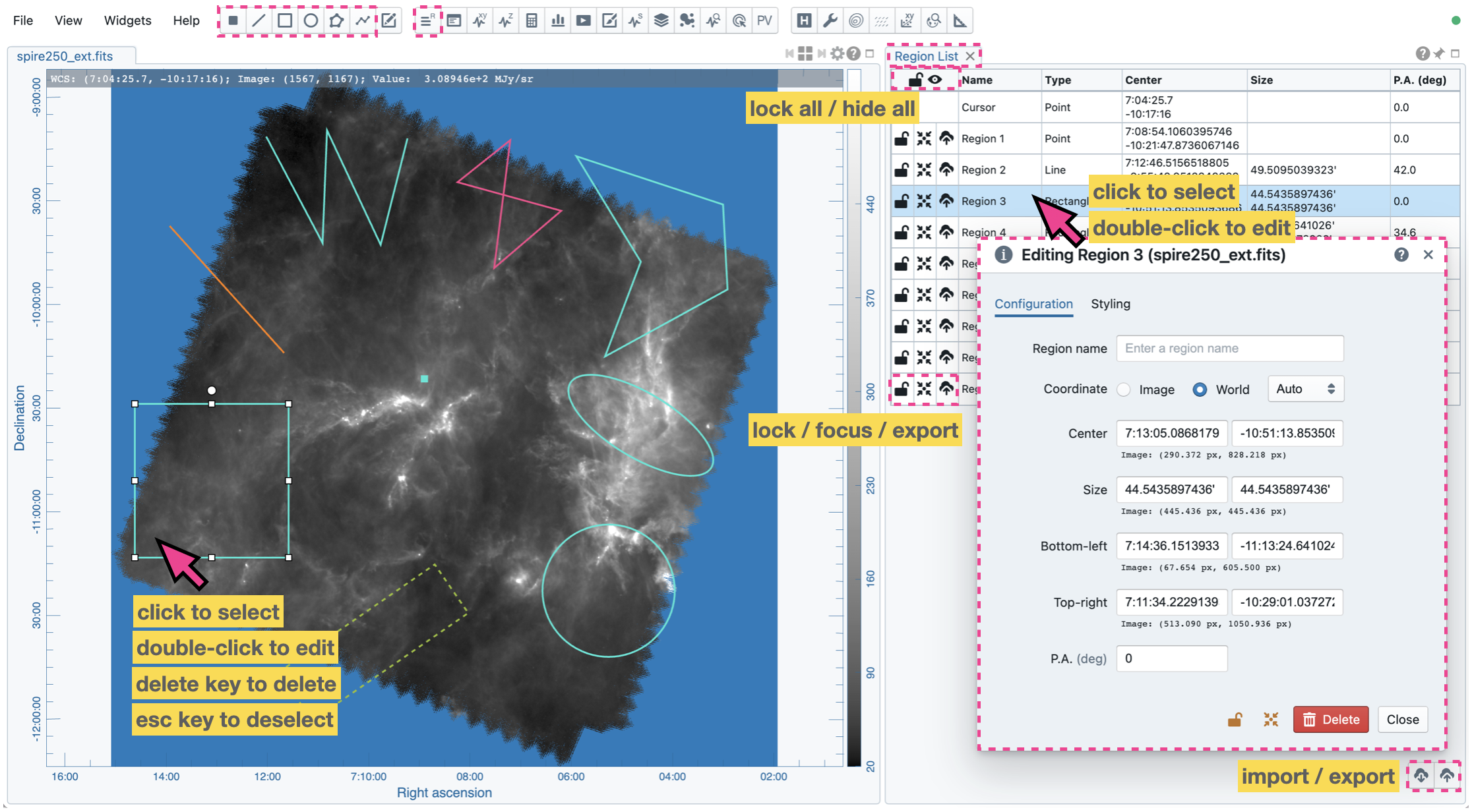
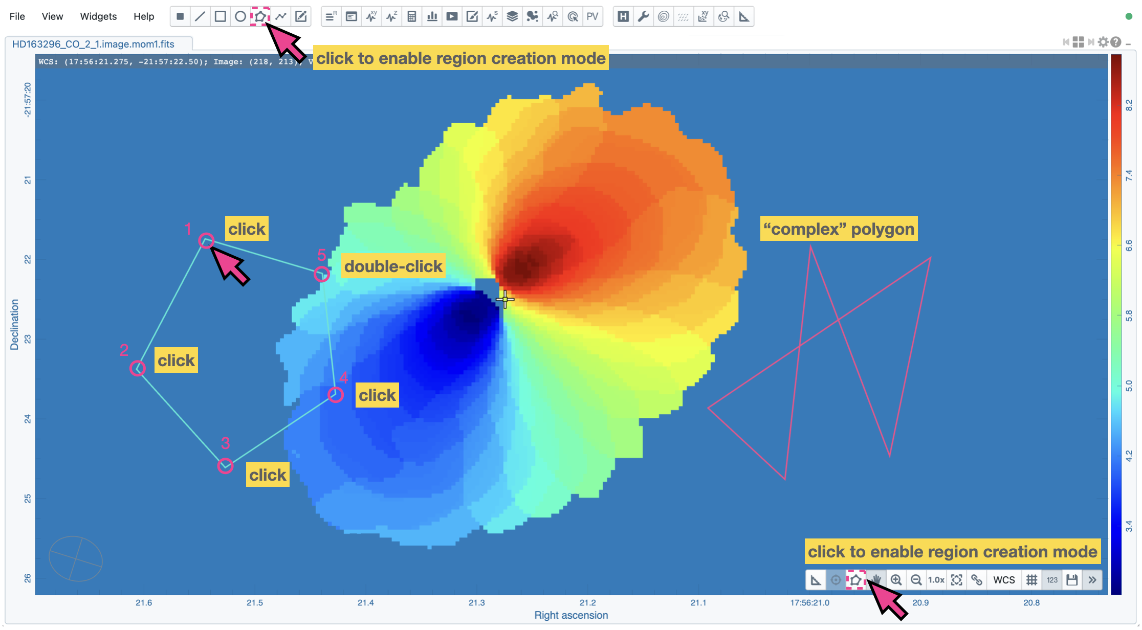
CARTA checks if a polygon is simple or complex. If a polygon is detected as complex (i.e., polygon line segments intersect), its color will become pink as a warning. Spectral profile, statistics, or histogram of a complex polygon can still be requested. However, the outcome may be beyond your expectations. The enclosed pixels depend on how a complex polygon is constructed. Please use complex polygons with caution.
The coordinate reference system can be changed with the dropdown menu when editing region properties in the world coordinates. The default reference system is the one defined in the image header and is the same as the one defining the grid line overlay in the Image Viewer. When you switch to a different reference frame, the Image Viewer’s grid line overlay is also changed. The coordinate is in sexagesimal format if the reference system is ICRS, FK5, or FK4. The coordinate is in decimal degrees if the reference system is GALACTIC or ECLIPTIC. The region size property can be defined in arcsecond with ", in arcminute with ', or in degrees with deg.
In case you would like to delete all regions at once, you can use the “delete” button at the bottom-right corner of the Region List Widget. A confirmation dialog will be shown to prevent accidental deletion.
Shared region with conserved solid angle#
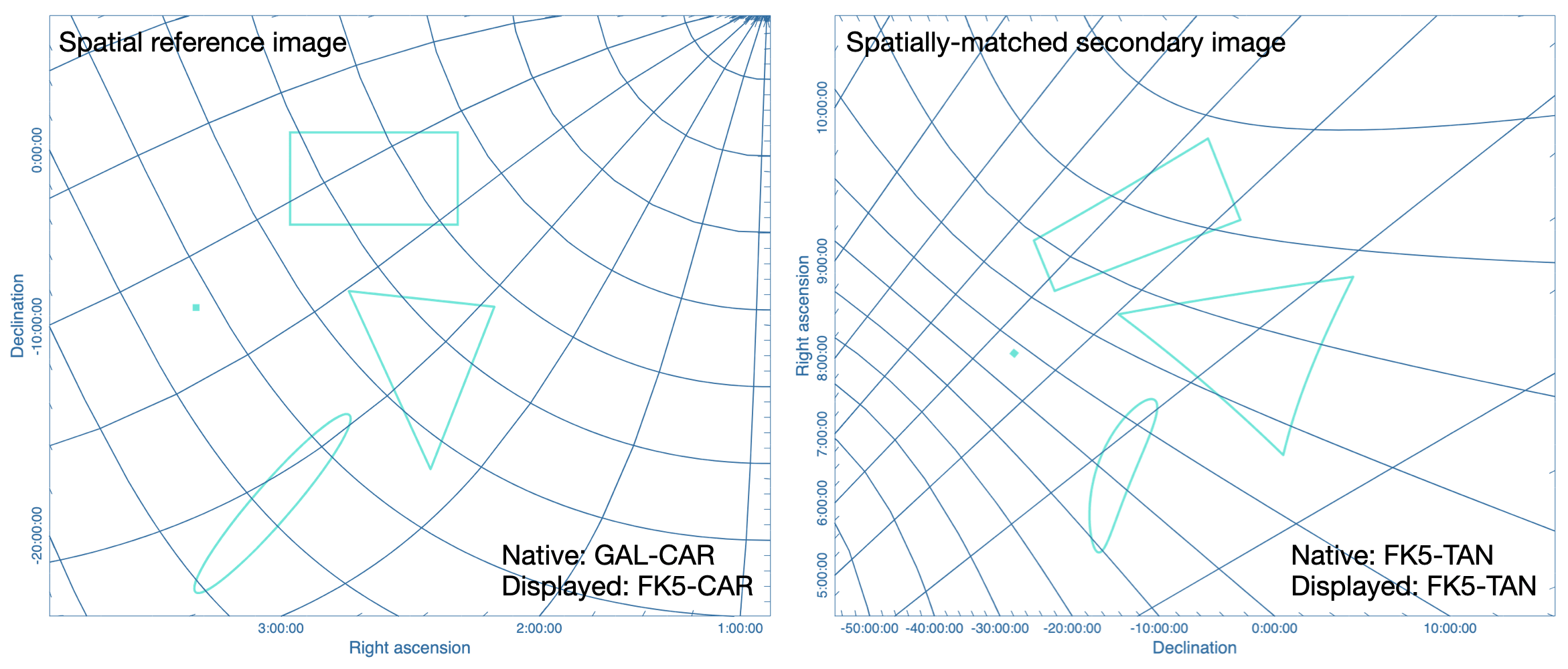
When a region is created on one of the spatially matched images, effectively, the region is created on the image served as the spatial reference. Then, the region is shared and rendered to other spatially matched images considering projection effects and differences in coordinate reference systems. Behind the scene, regions (except the point region) are approximated by polygons with many control points. Each control point is transformed from the spatial reference image to the spatially-matched secondary images. In this way, the solid angles of the regions before and after polygonal approximation are nearly identical; thus, analytics of the same region among different spatially matched images can be compared directly with minimal errors.
In the following exaggerated example, two images with different coordinate systems and projection schemes are spatially matched. Regions on the spatial reference image retain their shapes. Depending on the projection schemes, polygon-approximated regions on the spatially matched secondary images may have visible distortions. In most use cases, the region distortion effect should be much less noticeable if the field of view of the image is considerablely small.
Shared line/polyline region with conserved angular length#
Similar to the polygon approximation of closed regions, the line and polyline regions are approximated as a polyline with many control points on the spatially matched secondary images. In this way, the angular length of the trajectory traced by the line or polyline region before and after the polyline approximation is nearly identical.
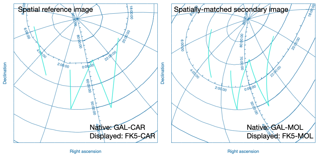
When a spatial profile is derived from a line or a polyline region, a set of boxes with a “height” (parallel to the trajectory) of three unit steps and a custom “width” (perpendicular to the trajectory) in the number of unit steps are created along the trajectory. These hidden boxes are created on the reference image first. Then, similar to the polygon approximation of closed regions, these “boxes” are transformed into the spatially matched secondary image to derive a spatial profile. The unit step refers to an image pixel if the image is “flat” without noticeable distortion. However, if the image is considered “wide” with noticeable distortion, the unit step refers to the angular size of an image pixel as defined in the image header (i.e. CDELT1/2). In this case, the boxes retain approximately a fixed solid angle. All these approximations allow spatial profiles of the same trajectory among different spatially matched images to be compared directly with minimal errors. The same idea is applied to the position-velocity image generator with a line region or a polyline region.
Shared region management#
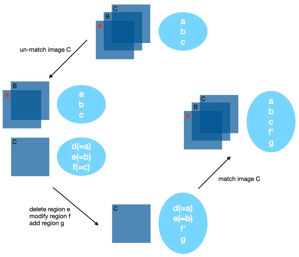
When regions are created on one of the spatially matched images, they are all registered to the spatial reference image for matching. The regions are shared with all the matched images; thus, analytics can be derived and compared directly. When an image is unmatched from the spatial reference image, the image will get a copy of all regions. This set of regions is now independent of the region set belonging to the matched images. Suppose there are modifications of the regions, and you try to match the image to the matched images again. In that case, only those modified regions will be copied to the region set of the matched images. The following diagram illustrates the idea.
Analytics with shared regions#
Shared region of interest enables practical image cube analysis through
Statistics Widget
Histogram Widget
Spectral Profiler Widget
Spatial Profiler Widget
Stokes Analysis Widget
PV Generator Widget
These widgets contain an “Image” dropdown menu and a “Region” dropdown menu. The former allows you to select which loaded image cube to show its analytics. The latter allows you to select which region to show the region analytics. By combining the two menus, CARTA provides a flexible user interface to explore image data. When the selected image has the polarization axis, you can use the “Polarization” dropdown menu to select which polarization component to use for deriving image analytics.
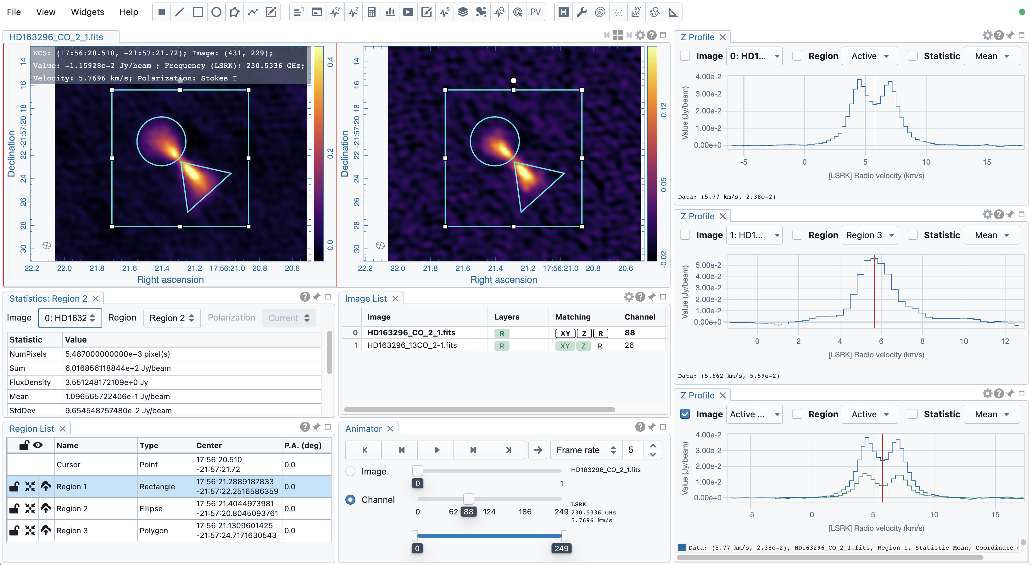
As an example below, two image cubes representing 12CO 2-1 and 13CO 2-1 are matched spatially and spectrally. Three shared regions are created to highlight different features. Three Spectral Profiler Widgets are placed to show different profiles. The top one shows the square region profile from 12CO 2-1. The middle one shows the polygon region profile of 13CO 2-1. The bottom one shows both 12CO 2-1 and 13CO 2-1 profiles from the square region. Please refer to the section Spectral profiler to learn how to plot multiple profiles in one Spectral Profiler Widget. In addition, one Statistics Widget is configured to show the statistics of 12CO 2-1 from the circle region.
Region import and export#
CARTA supports region import and export capability. In world coordinates or image coordinates, regions can be exported to a text file or imported from a text file. To import a region file, use the menu “File” -> “Import Regions”. A shortcut button can be found in the Region List Widget, too.
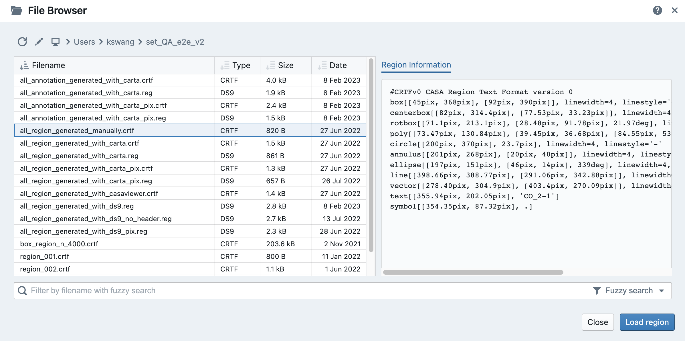
To export regions to a region file, use the menu “File”” -> “Export Regions”. A shortcut button can be found in the Region List Widget, as well. You can use the dialog to select a subset of regions to be saved in a region text file.
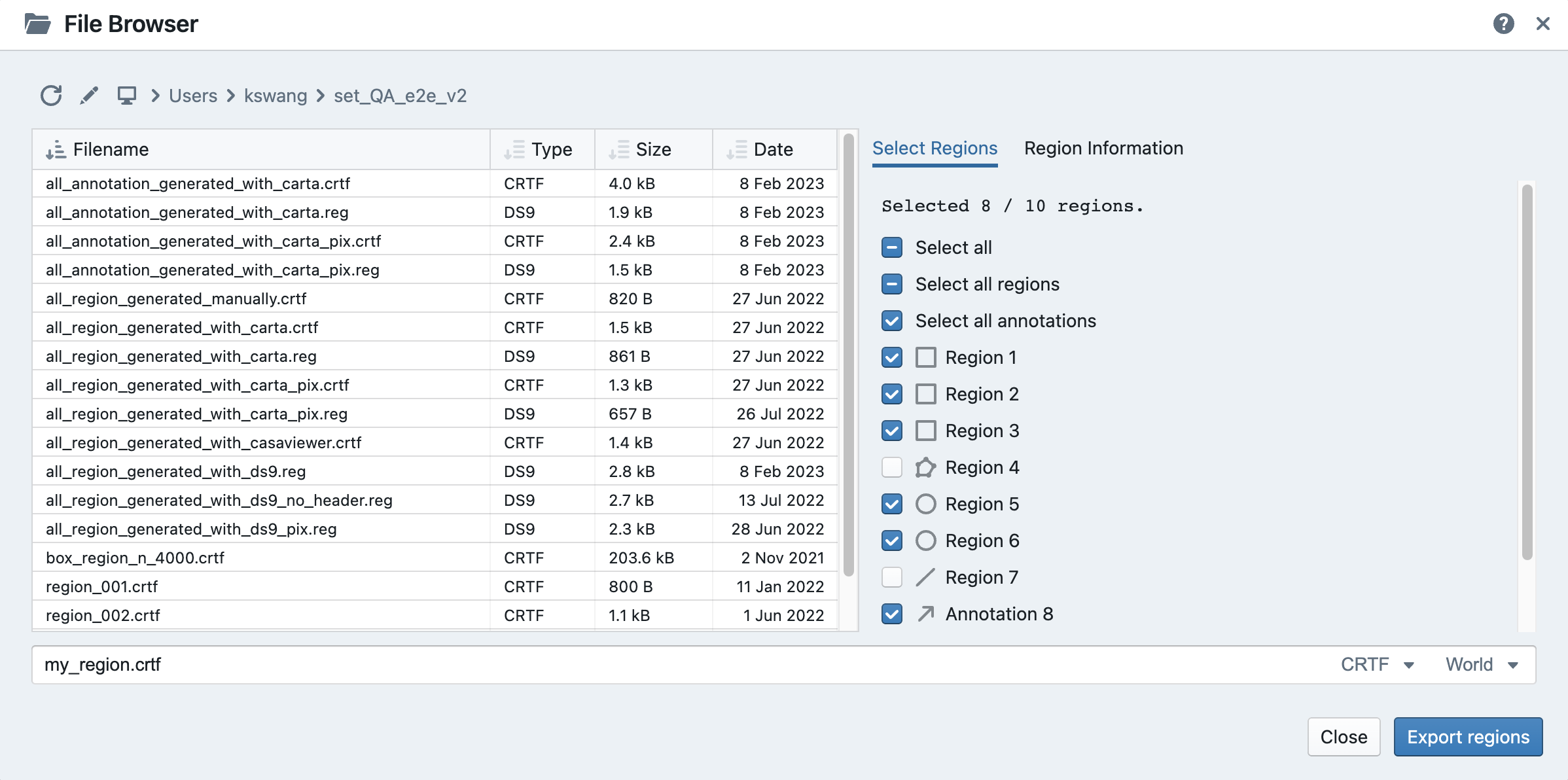
As of v6.0, CASA region text format (.crtf) and ds9 region text format (.reg) are supported with some limitations. Currently, only the 2D region definition is supported. Other properties, such as spectral range or reference frame, will be supported in future releases.
The supported CRTF region syntax is summarized below:
Rectangle
box[[x1, y1], [x2, y2]]centerbox[[x, y], [x_width, y_width]]rotbox[[x, y], [x_width, y_width], rotang]
Ellipse
circle[[x, y], r]ellipse[[x, y], [bmaj, bmin], pa]
Polygon
poly[[x1, y1], [x2, y2], [x3, y3], ...]
Polyline
polyline[[x1, y1], [x2, y2], [x3, y3], ...]
Line
line[[x1, y1], [x2, y2]]
Point
symbol[[x, y], .]
Please refer to https://casadocs.readthedocs.io/en/latest/notebooks/image_analysis.html#Region-File-Format for more detailed descriptions of the CRTF syntax.
The currently supported ds9 region syntax is summarized below:
Rectangle
box x y width height angle
Ellipse
ellipse x y radius radius anglecircle x y radius
Polygon
polygon x1 y1 x2 y2 x3 y3 ...
Polyline
polyline x1 y1 x2 y2 x3 y3 ...
Line
line x1 y1 x2 y2
Point
point x y
Please refer to http://ds9.si.edu/doc/ref/region.html for more detailed descriptions of the ds9 region syntax.
Image annotation#
Image annotation and region of interest share most attributes, except the ability for deriving image analytics. Image annotation is for presentation purposes only.
In CARTA, the following image annotation objects are supported:
point (with different marker shapes)
line (rotatable)
rectangle (rotatable)
ellipse (rotatable)
square (rotatable; as a special case of rectangle; “shift” key + drag)
circle (as a special case of ellipse; “shift” key + drag)
polygon
polyline
vector (rotatable)
text (rotatable)
compass
ruler
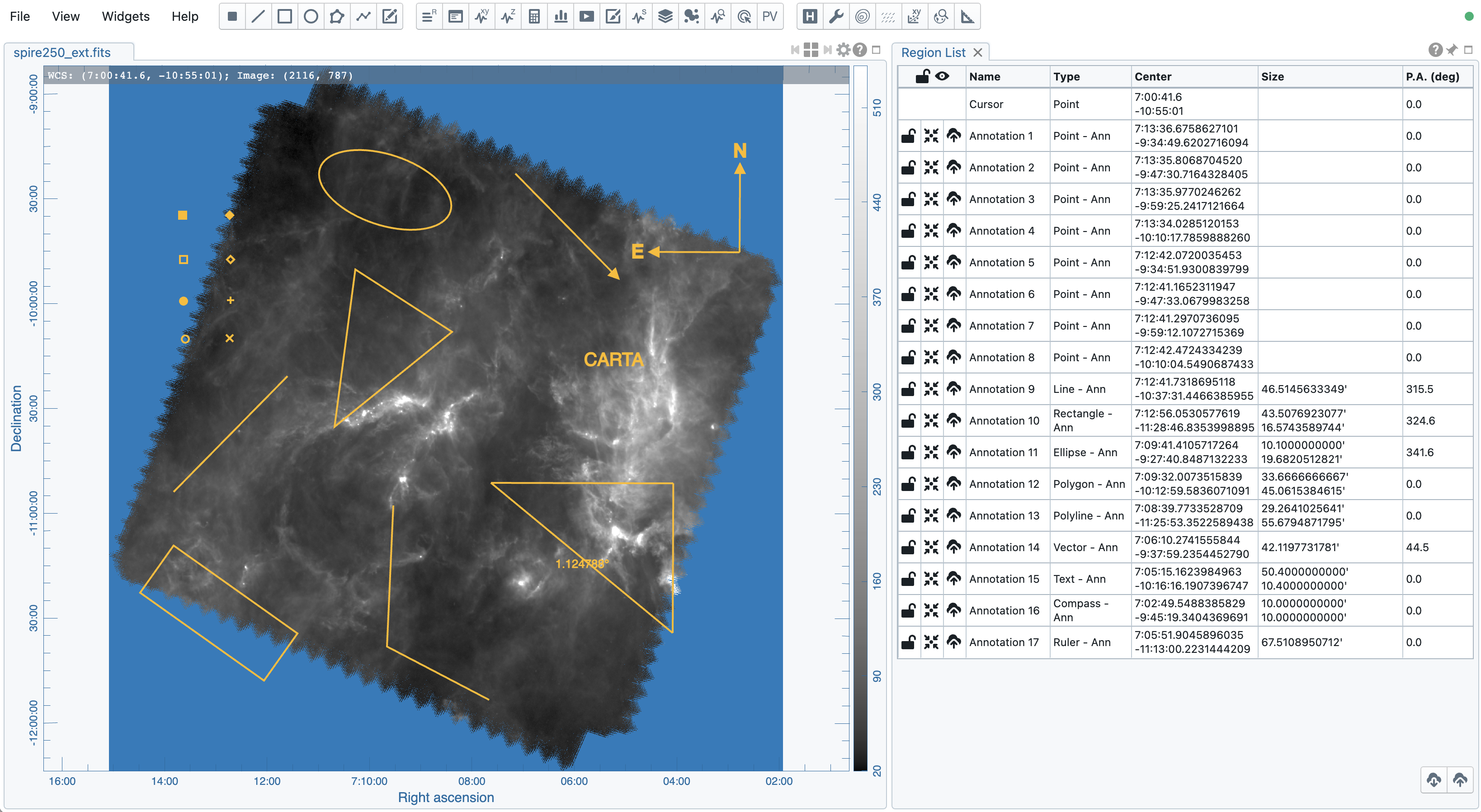
Image annotation objects created with the graphical user interface can be exported as a “region” text file in the CRTF or ds9 format.
What does “Active” mean?#
In CARTA, the term “active” is used to indicate the current focus of interaction. For example, an “active image” is the image (and a corresponding channel if it is an image cube) that is currently being viewed or analyzed in the Image Viewer as highlighted with a red box.
An “active region” is a region that has been selected and is ready for modification or analysis. The active state can be changed by clicking on the corresponding item in the GUI, such as an image in the Image Viewer / the Image List Widget or a region in the Image Viewer / the Region List Widget. When there is no region selected, the active region is defaulted to the “cursor” (a point) region.
When the active region does not refer to a closed region type such as a point or a line and if you request image statistics using the Statistics Widget, the statistics will be derived from the entire image instead. If you request a spectral profile but the active region refers to a line or a polyline, no profile will be derived and displayed.
A similar analogy applies to polarization dropdown menu (e.g., in the Spectral Profiler Widget) but the term is “current” which referes to the selection with the polarizarion slider in the Animator Widget.
Interacting with the graphical user interface#
The CARTA graphical user interface (GUI) is designed to be flexible and user-friendly, supporting a variety of use cases such as continuum image analysis, spectral line cube analysis, polarization cube analysis, and catalog analysis. This section introduces the GUI and provides examples to familiarize you with layout configuration via mouse actions and how to interact with images, regions, and charts.
Components#
The CARTA GUI has different components:
Main browser window
Menu bar
Region bar
Widget bar
Dialog bar
Status bar
Toolbar
Widget (docked)
Widget (floating)
Tab
Dialog
Popout Image Viewer browser window
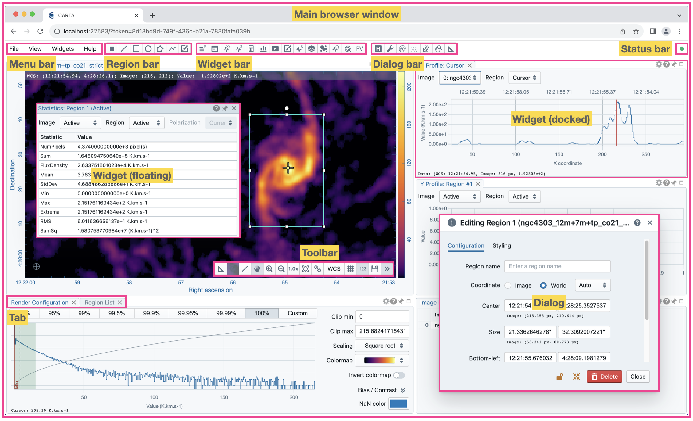
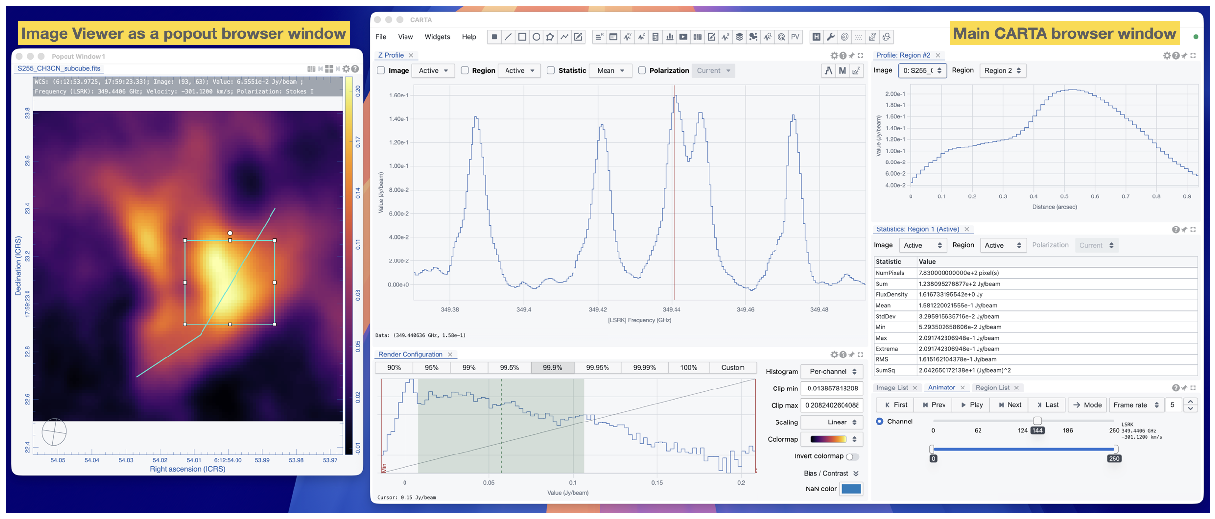
The main browser window consists of a set of docked widgets. Multiple docked widgets can be stacked and share the same space. In this case, inactive widgets are displayed as tabs. For example, the figure above shows five docked widgets in the main browser window. Among them, two docked widgets share the same space as tabs (render configuration and region list) in the bottom-left part of the GUI. A docked widget (i.e., a tab) may be detached to become a floating widget by clicking the “pin” button at the top-right corner of the widget (widget control buttons). The GUI layout is highly configurable via mouse and is reusable. Please refer to the section Configuring the layout for details.
The menu bar provides control options, such as image input/output, launching widgets, getting help, etc. The widget bar provides widgets to view or analyze images. The dialog bar provides dialogs for configurations. The region bar provides shortcut buttons for creating regions of interest or image annotation objects in the Image Viewer.
The status bar includes indicators of the server (backend) status (as a green, orange, or red circle), data stream status (as a green cloud), new release notification (as an orange envelope), and share workspace button (“Site Deployment Mode (SDM)” only).
A widget provides a specific function to view or analyze image data, such as Image Viewer, Statistics, Spatial Profiler, etc. A toolbar provides tools for a widget, such as zoom buttons for the Image Viewer Widget or export options for the Spectral Profiler Widget. A dialog provides options for configurations, such as image view properties, region properties, contour properties, etc.
As a new feature in v6.0, the Image Viewer can be popped out to a new browser window. This feature is useful when you want to view images on a secondary monitor, while keeping the main browser window for analytics widgets. Using the popout button in the top-right corner of the Image Viewer, you can pop out the Image Viewer to a new browser window. The popped-out Image Viewer can be resized and moved freely, just like a regular browser window. The popped-out Image Viewer can be restored by clicking the close button of the browser window.
Note
When the Image Viewer is popped out to a new browser window, saving a layout configuration or saving a workspace is forbidden. Please restore the Image Viewer to the main browser window before saving a layout configuration or saving a workspace.
Server-side status and session resume#
As CARTA is fundamentally a client-server application, it would be essential to know the status of the server side at the client side (i.e., your web browser). It is also helpful to know whether the standalone version runs normally. The server (i.e., the carta_backend) status is displayed as a circular icon in the top-right corner of the main browser window. The connection latency and a session ID can be seen by hovering over the icon. There are three kinds of status:
Green: This means that the server side is connected successfully.
Orange: This means that the initial connection to the server side was broken (e.g., unstable internet) but has been reconnected. You will be asked to resume the previous session or not.
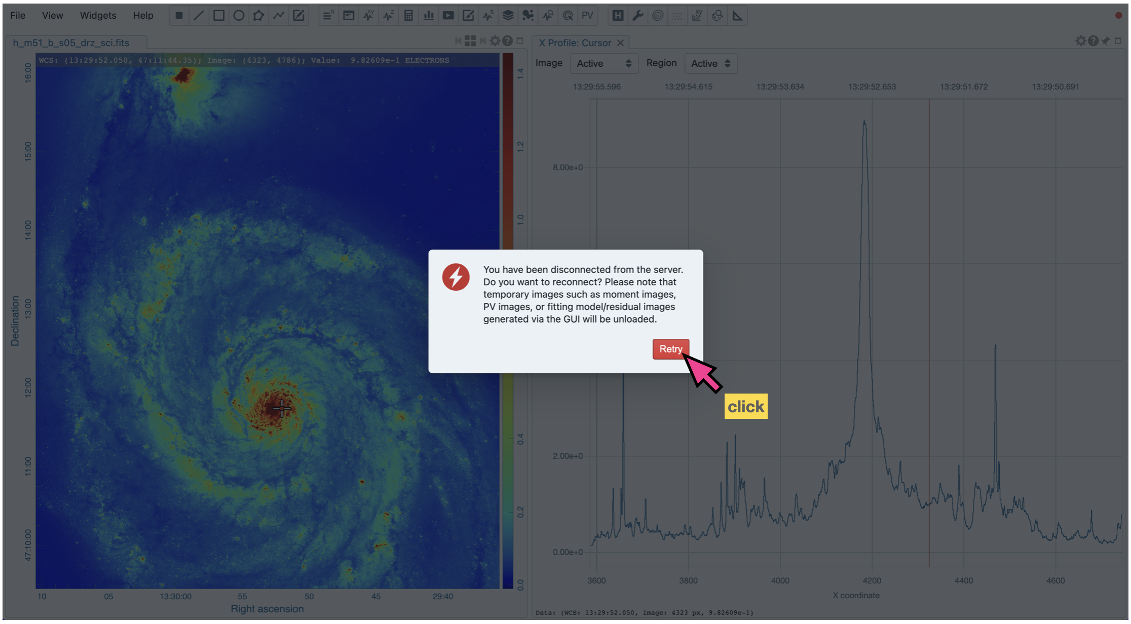
Red: This means that the server side is not accessible, either due to a broken internet or a backend crash. CARTA is not functional in this case.
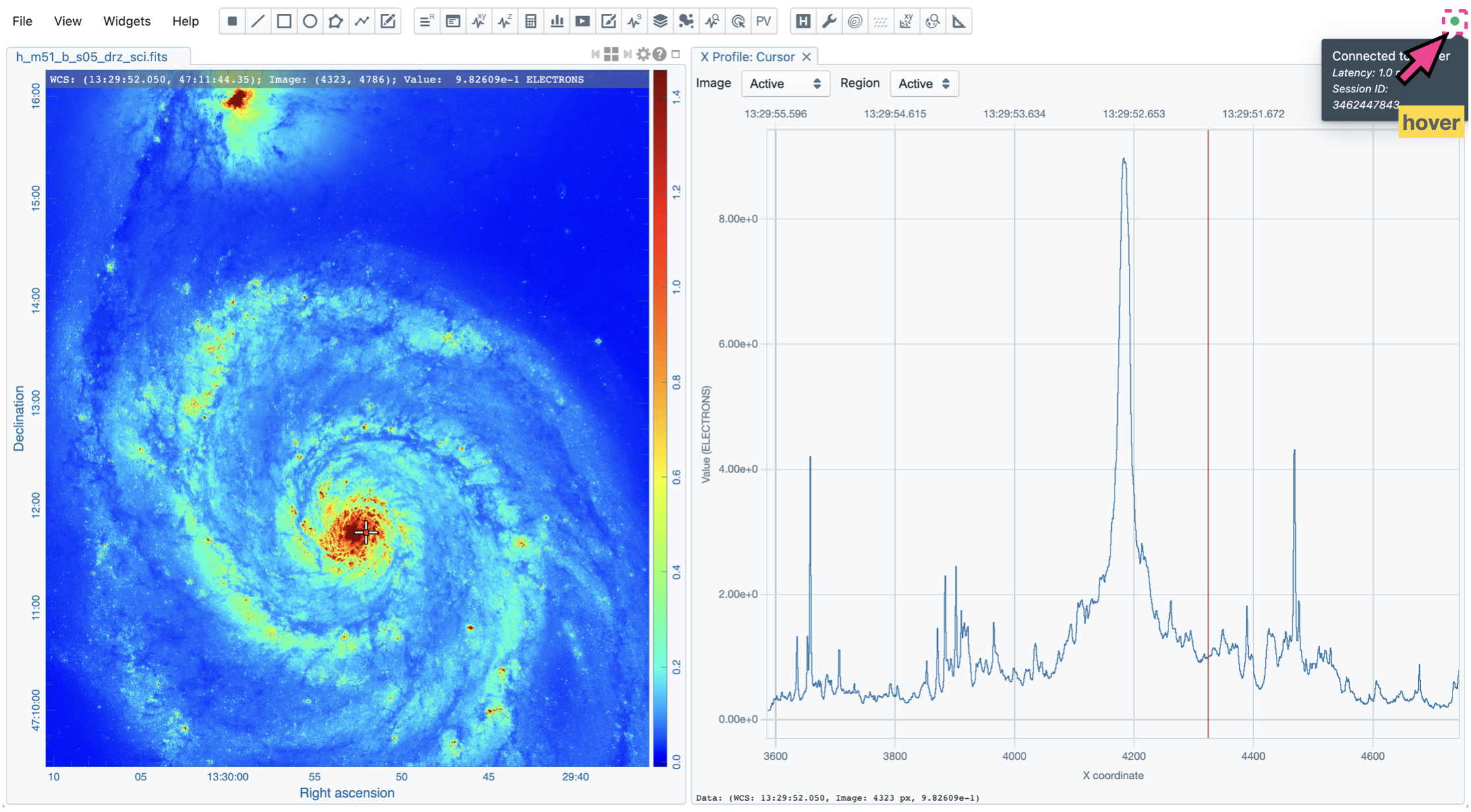
If CARTA behaves abnormally or stops responding, please check the server-side status icon and the connection latency. If it becomes red, the connection between the client and server sides is interrupted. At this point, CARTA is not functional. A prompt will be shown in the browser to ask you whether or not to resume the previous CARTA session. By clicking the “Retry” button, CARTA will try to resume the previous session if possible. If you choose not to resume the previous session, please reload CARTA to establish a new session.
If you are using the Site Deployment Mode (SDM) of CARTA and encountering the case that the backend is not accessible, you can go to the dashboard to restart a CARTA service. The dashboard can be also visited also via the menu “File” -> “Server” -> “Dashboard” in normal state. With the dashboard, you can
Start a new CARTA session (using the same backend)
Restart a CARTA service (a.k.a., backend)
Show backend log
Logout
Note that the dashboard may look differently per site deployment.
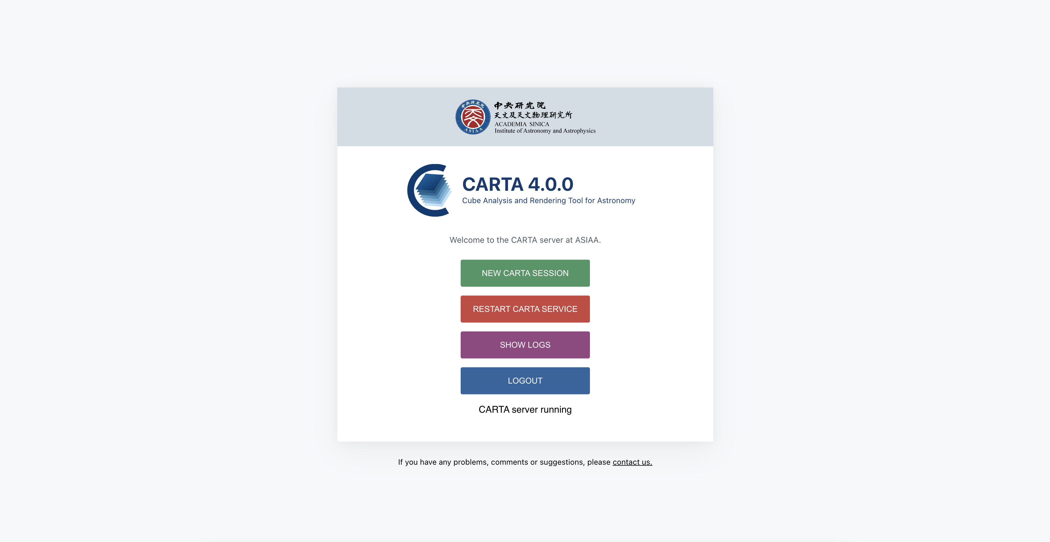
Image view interactions#
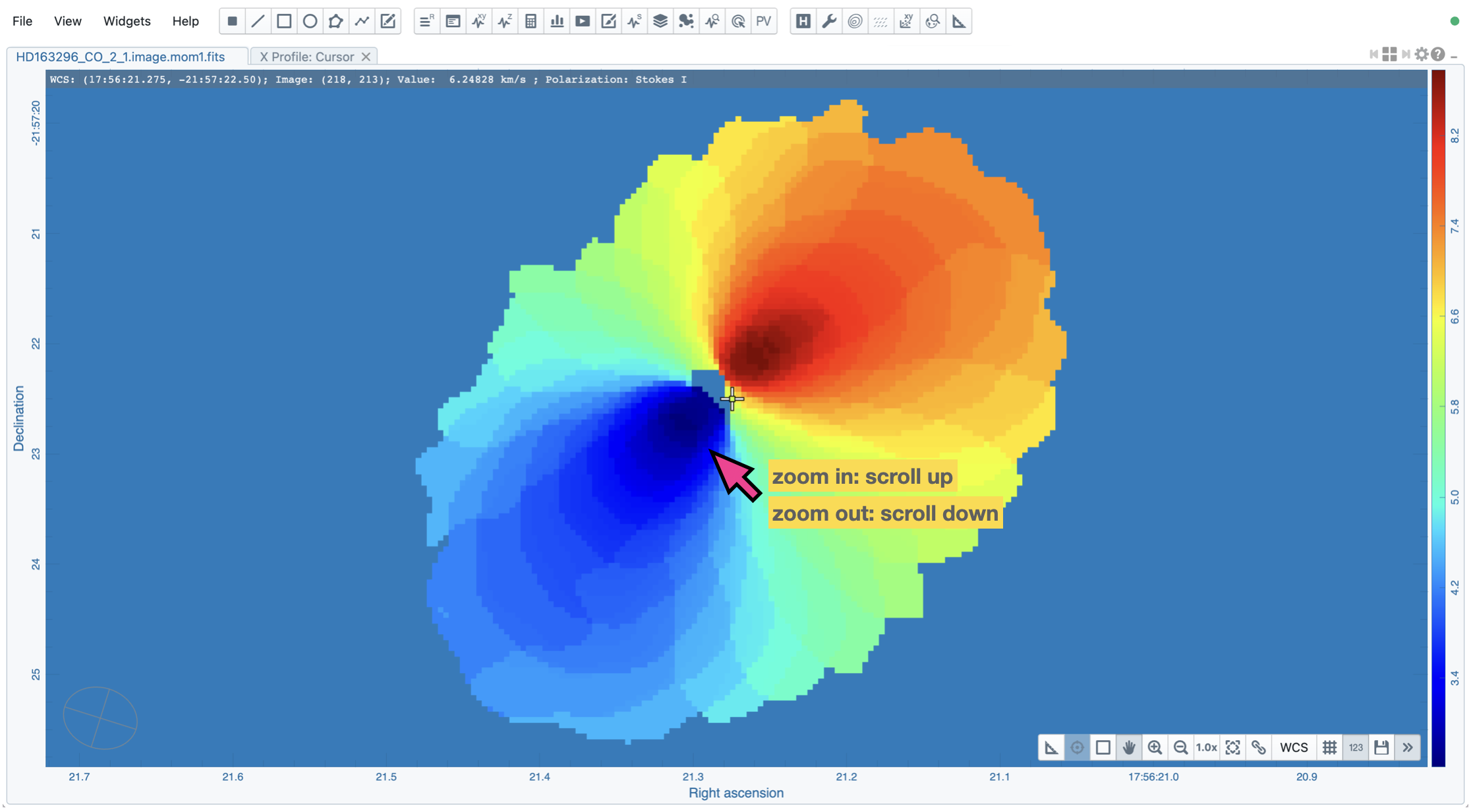
To zoom an image
Use the mouse wheel to scroll
Use the zoom buttons from the toolbar of the Image Viewer
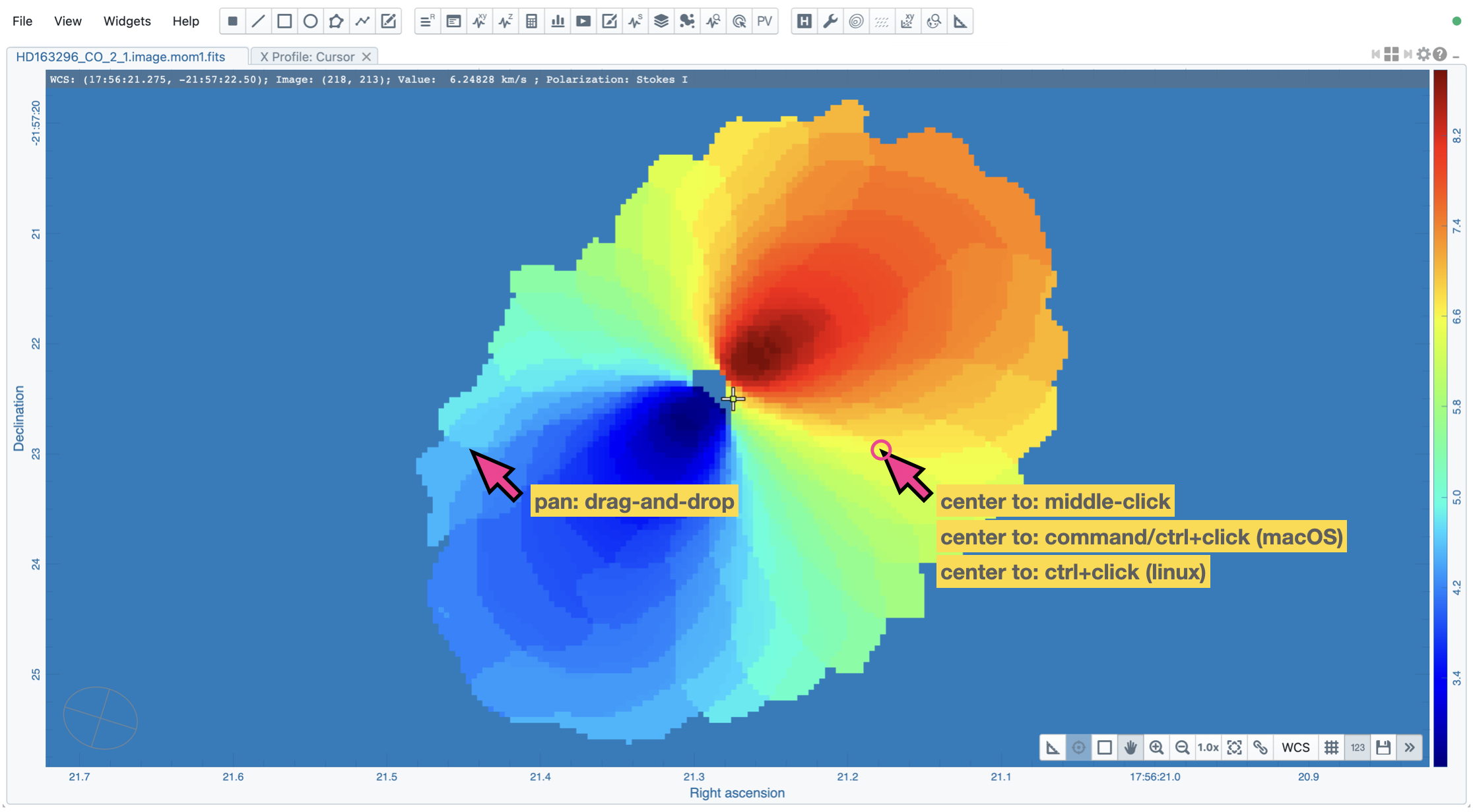
To pan an image
Use the mouse to drag-and-drop on the image (default)
Hold the “command” (macOS) / “ctrl” (Linux) key, then mouse click
Mouse middle click
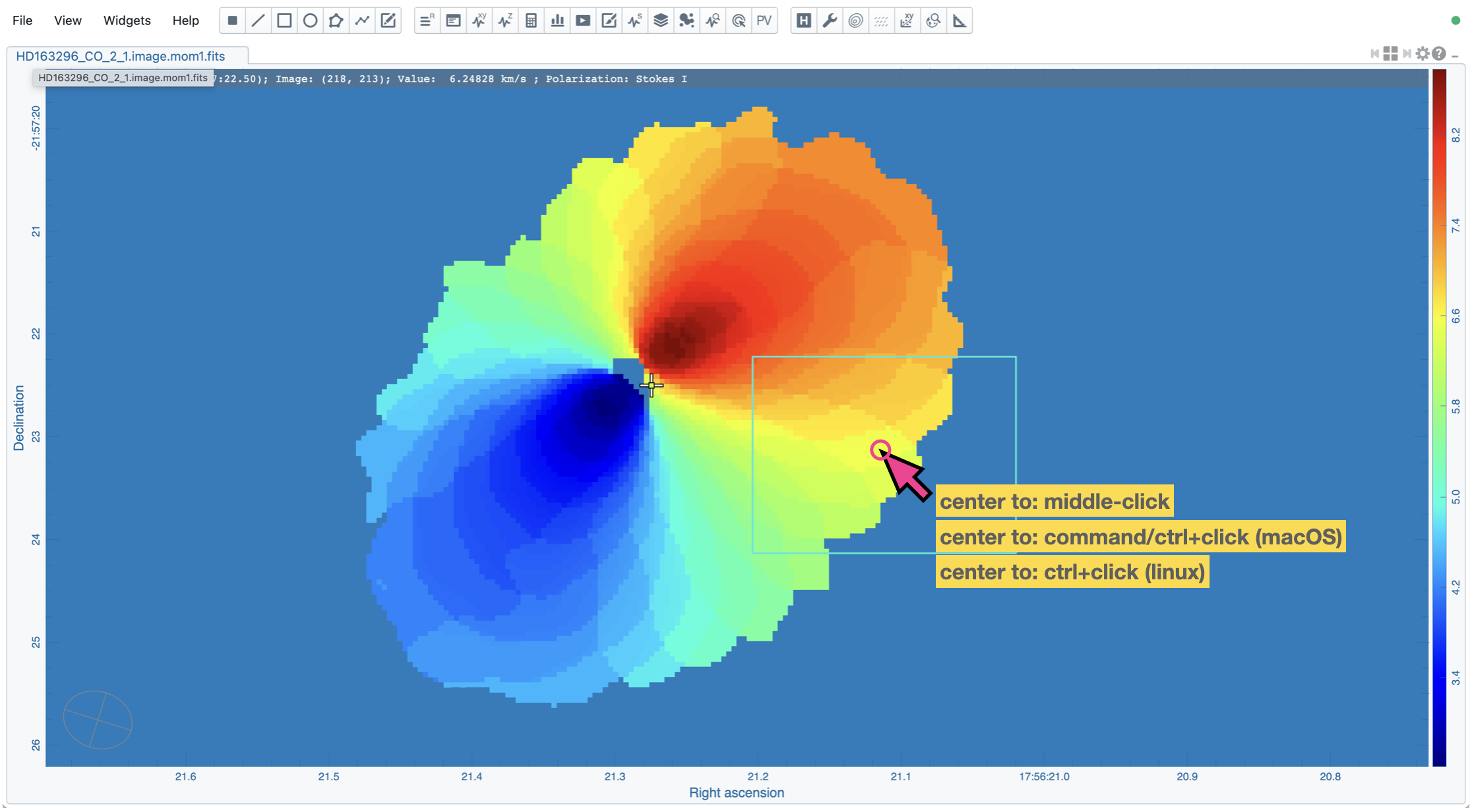
To pan from inside a region
Mouse middle click
If the region is locked, hold the “command” (macOS) / “ctrl” (Linux) key, then mouse click
Region of interest or image annotation object interactions#
Regions of interest and image annotation objects share similar behaviors. In the following, we use “region” for short.
Summary
To enable region creation mode
Press the “C” key
Click the region creation button from the toolbar of the Image Viewer
Click a target region type from the region bar
To create a circle region via the ellipse region type or a square region via the rectangle region type
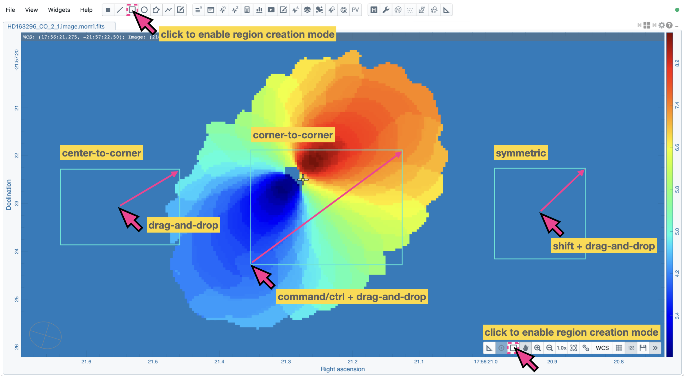
Hold the “shift” key, then drag-and-drop
To multi-select regions
In the image viewer, hold the “shift” key, then click-and-drag a box to enclose the regions
In the image viewer, hold the “command / ctrl” key, then click on the regions
In the region list widget, hold the “command / ctrl / shift” key, then click on the regions
To create or modify a region (rectangle, ellipse, or line) with the alternative mode (center-to-corner v.s. corner-to-corner)
Hold the “command” (macOS) / “ctrl” (Linux) key, then drag-and-drop
To configure a region
Double-click on a region entry in the Region List Widget
Double-click inside a region in the Image Viewer
To lock/unlock a region
Press the “L” key
Press the “shift” + “L” key to unlock all locked regions
Click the lock button in the Region List Widget
Click the lock button in the Region Configuration Dialog
To delete a region
Press the “delete” key
Press the “backspace” key
Click the delete button in the Region Configuration Dialog
Regions of interest and annotation objects share similar behaviors. In the following, we use “region” for short.
Region creation
A region can be created by entering the region creation mode and then applying drag-and-drop action in the Image Viewer. To enter the region creation mode, click the “region” button in the bottom-right corner of the Image Viewer or press the “C” key. Double-clicking the region icon brings up all available region types (rectangle, ellipse, polygon, point, line, and polyline). Alternatively, you may click the buttons in the region bar at the top of the GUI to enter the region creation mode.
To create a point region, a single click will do. The rectangle region, the ellipse region, or the line region can be created in the “center-to-corner” mode or the “corner-to-corner” mode, depending on the preferences setting in the Preferences Dialog (”File” -> “Preferences -> “Region”). To temporarily switch to the other mode, hold the “command” (macOS) or “ctrl” (Linux) key then drag-and-drop. The “circle” and the “square” regions are the special cases of the ellipse region and the rectangle region, respectively. These symmetric regions can be created by holding the “shift” key followed by the drag-and-drop action. Alternatively, a single mouse click can create a rectangle region, an ellipse region, or a line region. The default size on the screen is defined in the Preferences Dialog (”File” -> “Preferences” -> “Region”).
To create a polygon region or a polyline region, start with a click followed by a series of clicks to define the control points of a desired shape and finish with a double click. CARTA detects a “complex” polygon (polygon with intersections) and shows it in pink. Spectral profiles, statistics, or histograms of a complex polygon can still be requested. However, please note that the results may be beyond your expectations since the actual pixel coverage depends on how a complex polygon is created.
Region selection and modification
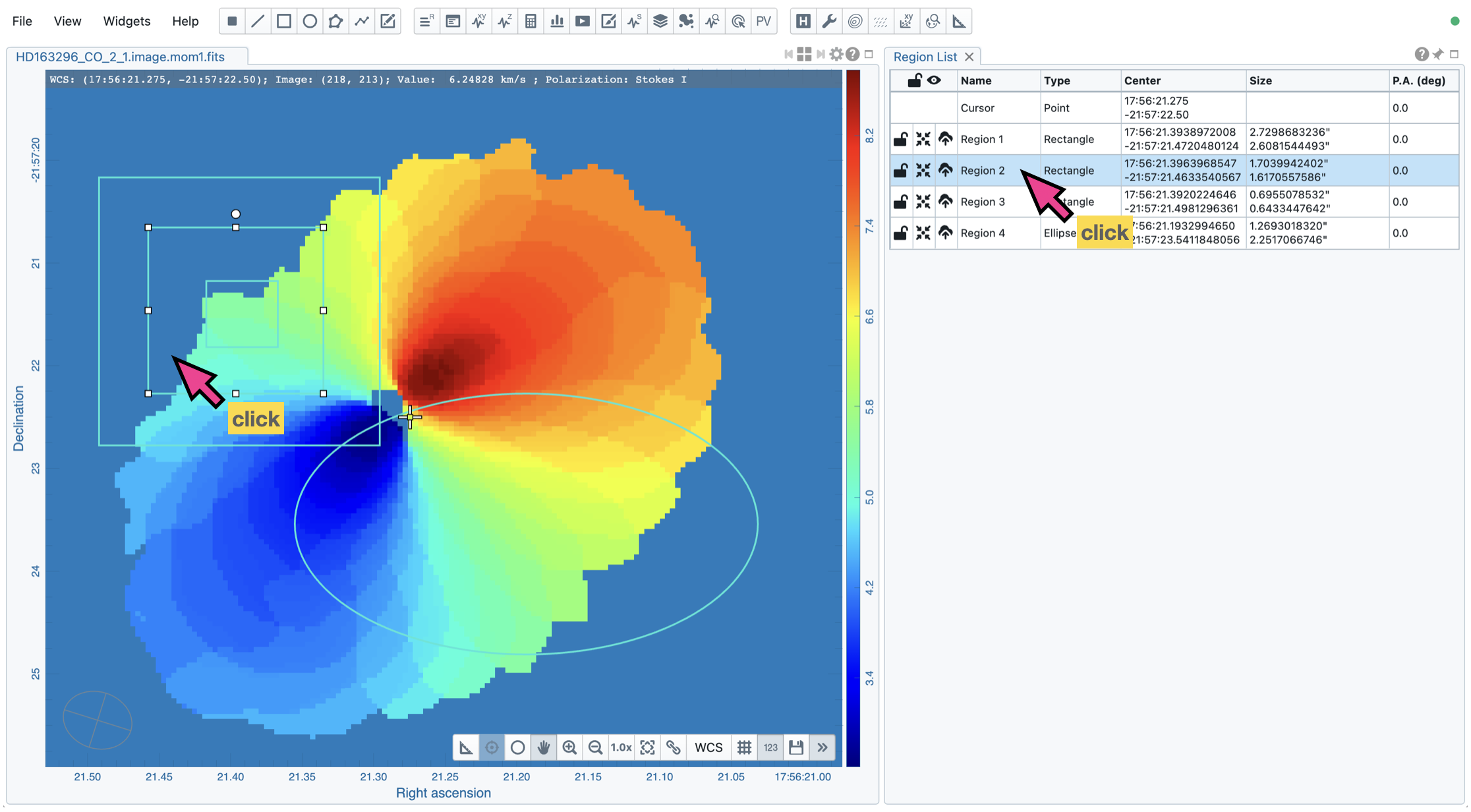
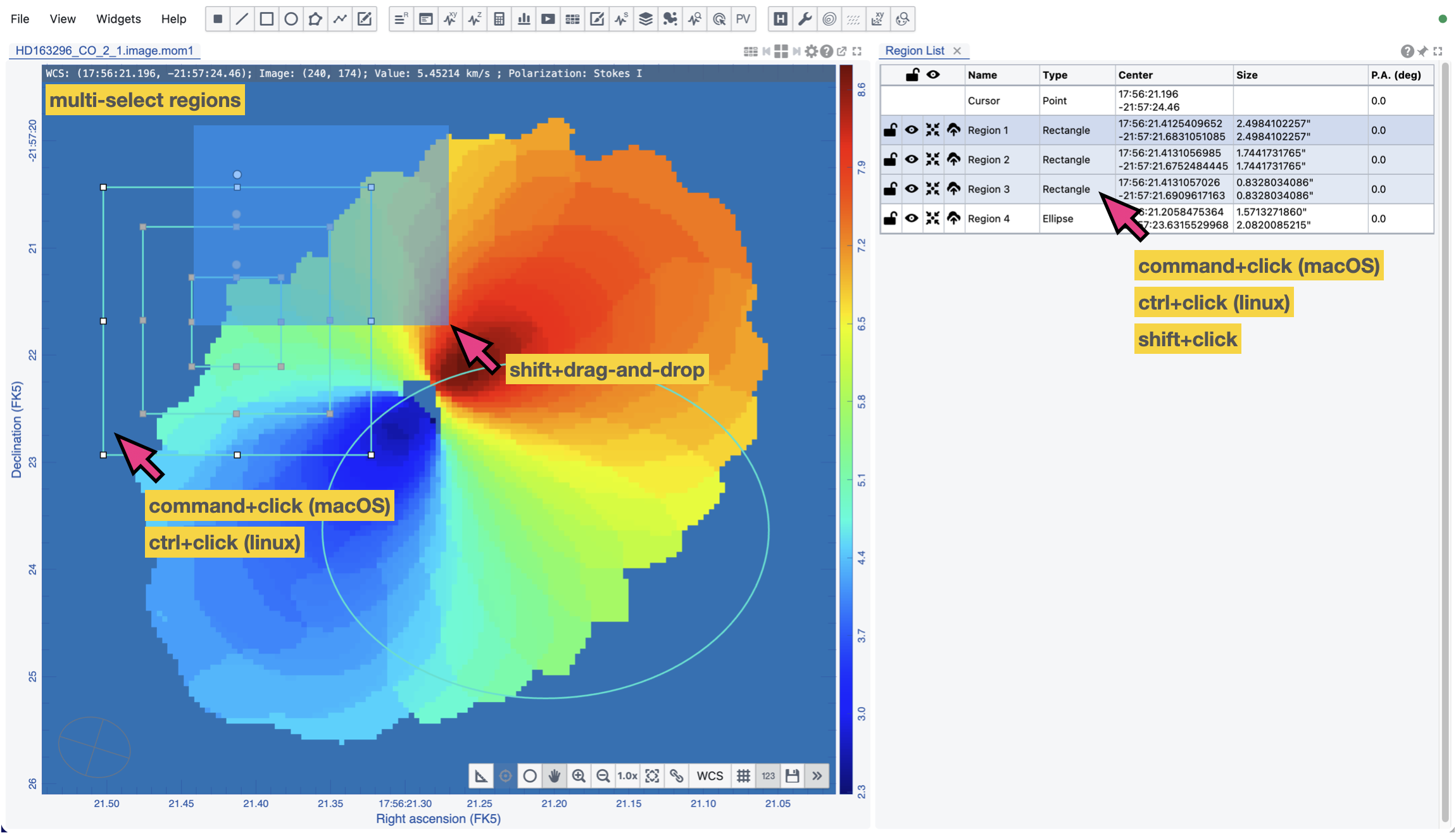
Click on a region in the Image Viewer will change the region state to “active”. The active region will be highlighted in the Region List Widget. Alternatively, a region can be selected by clicking a region entry in the Region List Widget. Multi-selection of regions is also supported. In the Image Viewer, hold the “shift” key and click-and-drag a box to enclose the regions, or hold the “command / ctrl” key, then click on the regions. In the Region List Widget, hold the “command / ctrl / shift” key, then click on the regions.
CARTA allows selecting a “region in region”. The layer order of regions is adjusted automatically based on the region size. To deselect a region, click elsewhere in the Image Viewer or press the “esc” key.
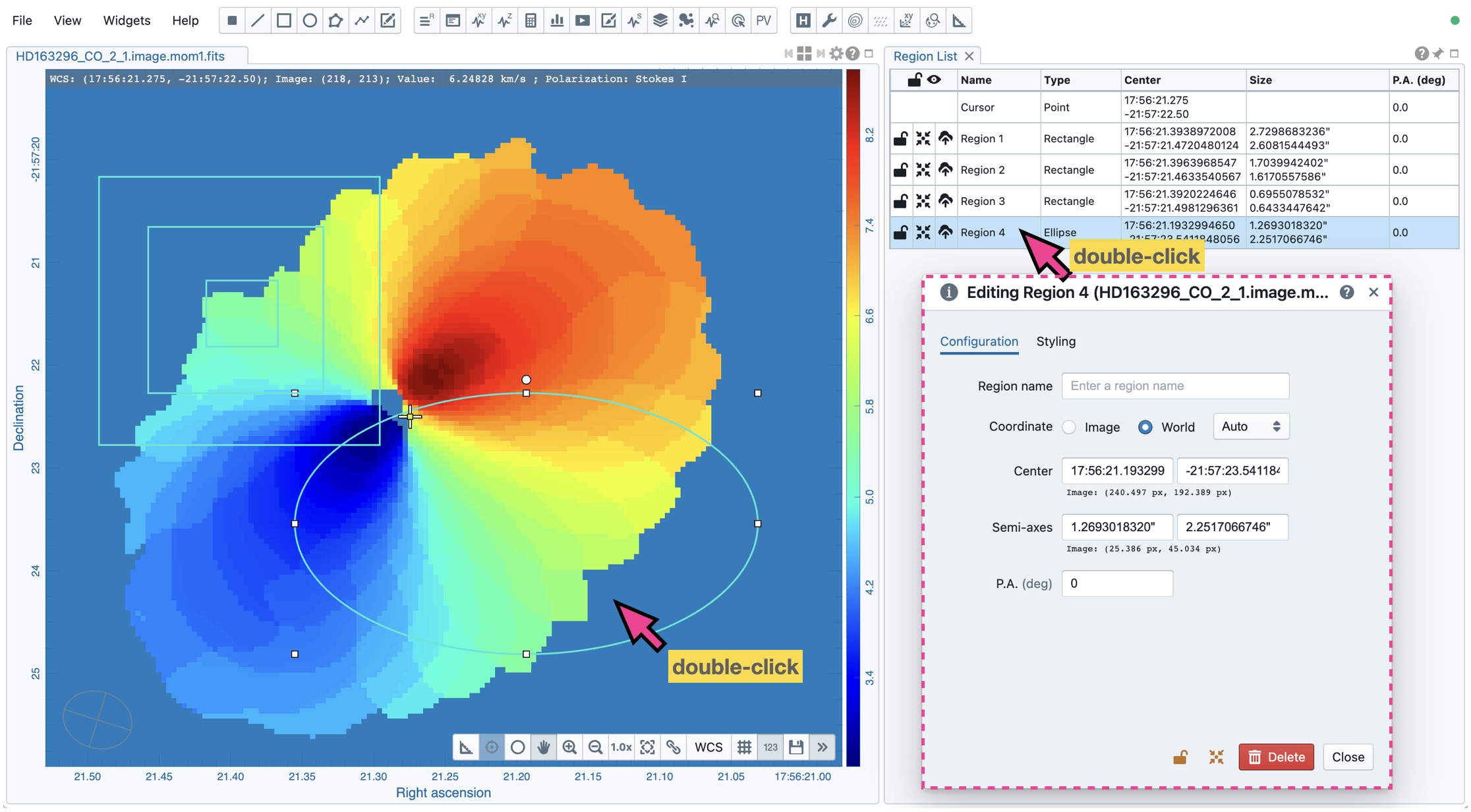
Double-click on a region in the Image Viewer or a region in the Region List Widget will launch the Region Configuration Dialog. You can make changes to the region’s name, location, shape, and style using the dialog. When multiple regions are selected, the Region Configuration Dialog will display the common properties only. Pressing the “delete” or the “backspace” key will remove the active region or selected regions.
Tip
“backspace” does not delete a region…
When you launch CARTA with the Firefox web browser on macOS, you may find the “backspace” key navigates back a page instead of removing a region. This behavior can be prevented by modifying your Firefox web browser settings:
Enter about:config in the address bar.
Click “I accept the risk!”
A search bar appears at the top of a long list of preferences. Search for “browser.backspace_action”
It will likely have a value of 0. Double-click it, and then modify it to a value of “2”.
Close the about:config tab, and now backspace will no longer navigate back a page.
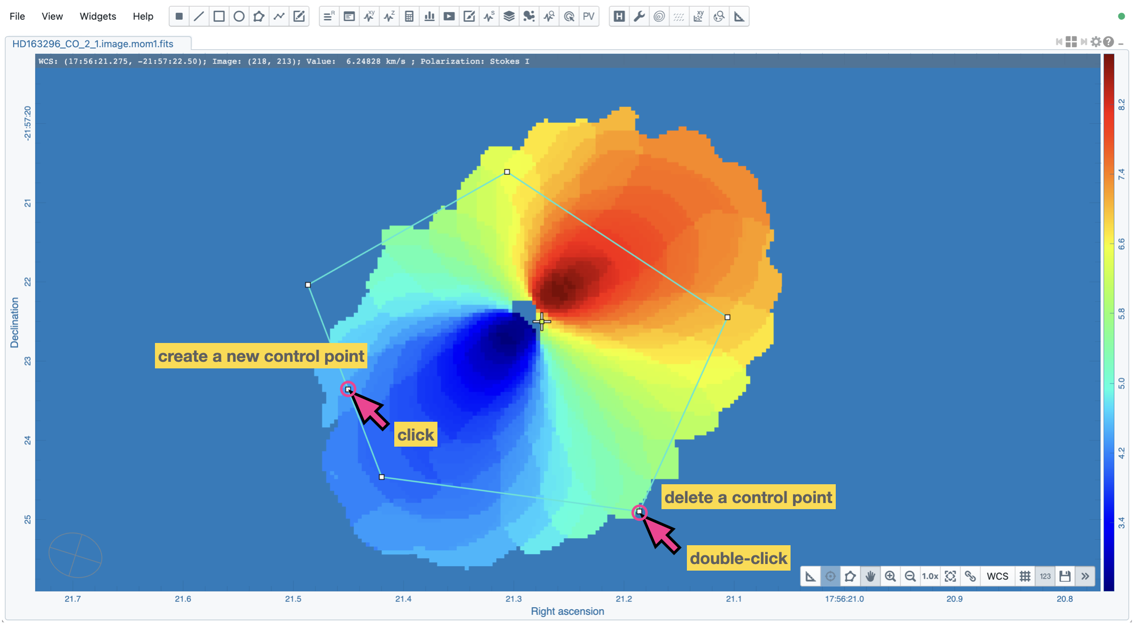
A new control point can be added by double-clicking on a line segment for a polygon or polyline region. A control point can be deleted by double-clicking on the control point.
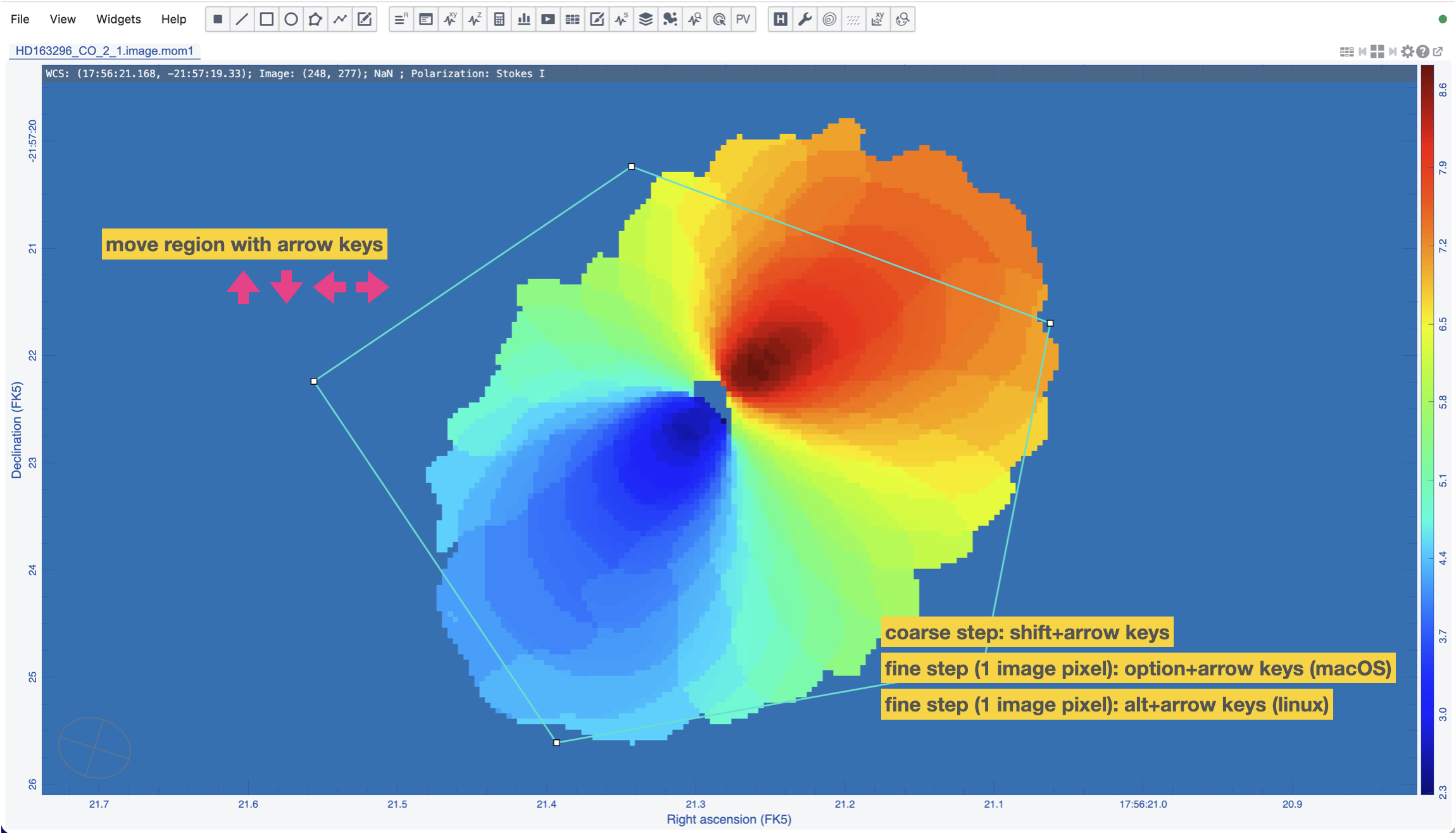
Move region with keyboard
To move a selected region with the keyboard, use the arrow keys for the default step (in screen pixel), hold the “shift” key and use the arrow keys for the coarse step (in screen pixel), or hold the “option” (macOS) / “alt” (Linux) key and use the arrow keys for the fine step (one image pixel).
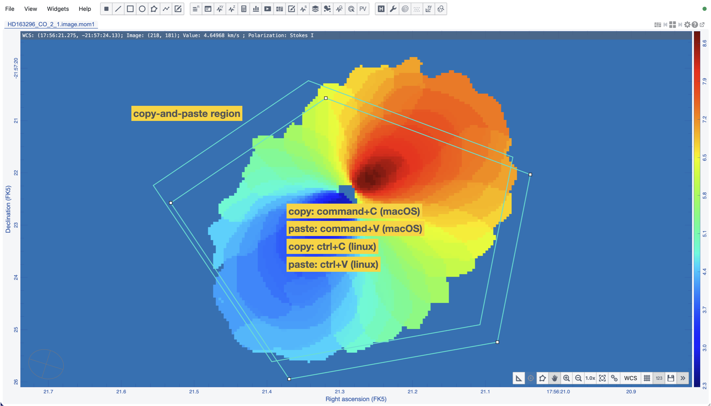
Copy and paste a region or regions
To copy a region or regions, select the region or regions and press the “command” + “C” key (macOS) or the “ctrl” + “C” key (Linux). To paste a region or regions, press the “command” + “V” key (macOS) or the “ctrl” + “V” key (Linux).
Fine keyboard control of region control points
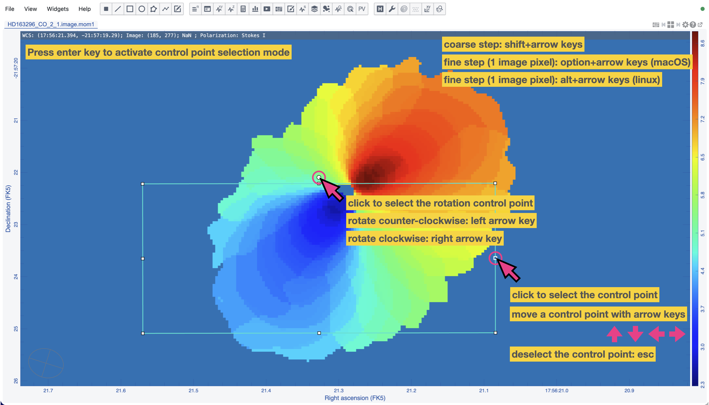
A control point of a region can be selected by clicking on it. The selected control point can be moved with the arrow keys for the default step (in screen pixel), hold the “shift” key and use the arrow keys for the coarse step (in screen pixel), or hold the “option” (macOS) / “alt” (Linux) key and use the arrow keys for the fine step (one image pixel). Alternatively, a control point can be selected by pressing the “enter” key when a region is selected. To cycle through other control points of a region when a control point is selected, press the “tab” key or “shift” + “tab” key. To deselect a control point, press the “esc” key. When a rotation control point is selected, pressing the “left” key to rotate counter-clockwise and the “right” key to rotate clockwise. Similarly, the “shift” key can be held to rotate in a coarse step and the “option” (macOS) / “alt” (Linux) key can be held to rotate in a fine step.
Cursor update#
To freeze or unfreeze cursor position update in the Image Viewer
Press the “F” key
To show/hide cursor marker rendering
Press the “G” key
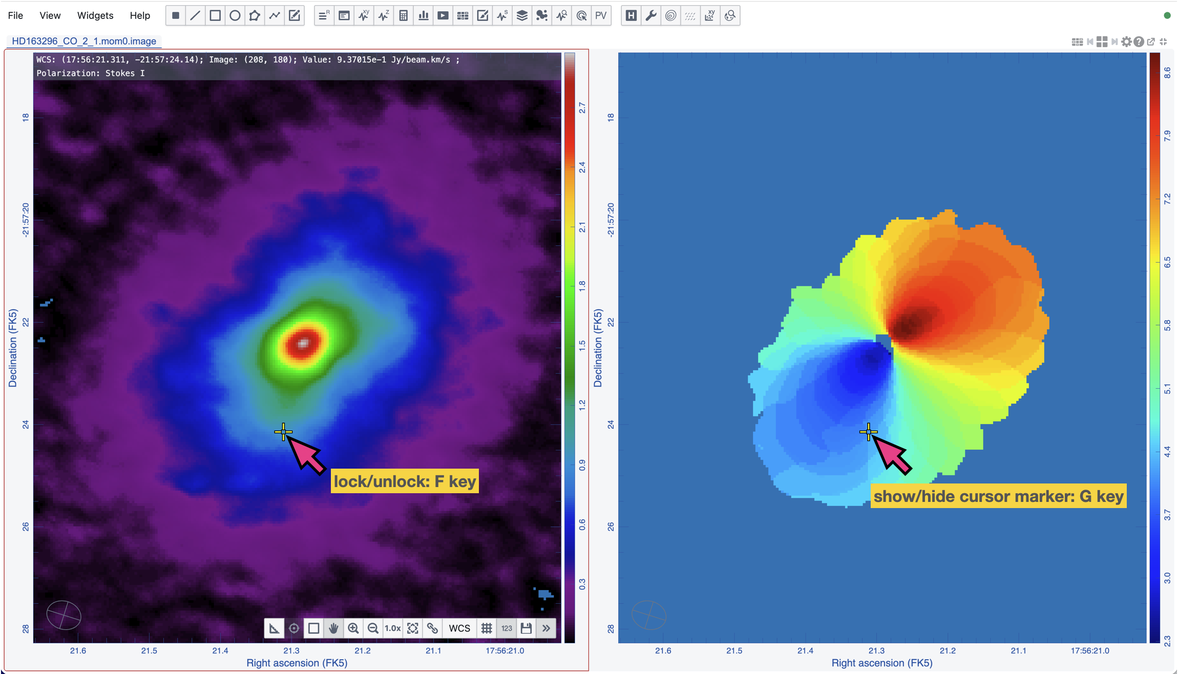
Chart interactions#
Summary
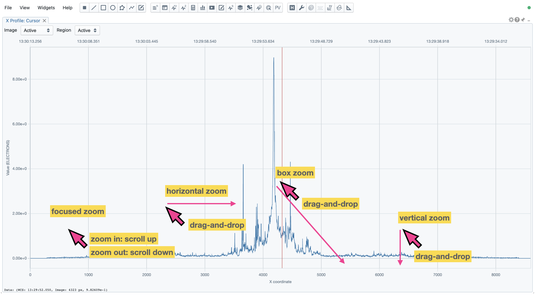
Focused zoom
Use the mouse wheel to scroll
Horizontal zoom
Drag-and-drop in the horizontal direction
Vertical zoom
Drag-and-drop in the vertical direction
Box zoom
Drag-and-drop in the diagonal direction
Reset zoom
Double-click
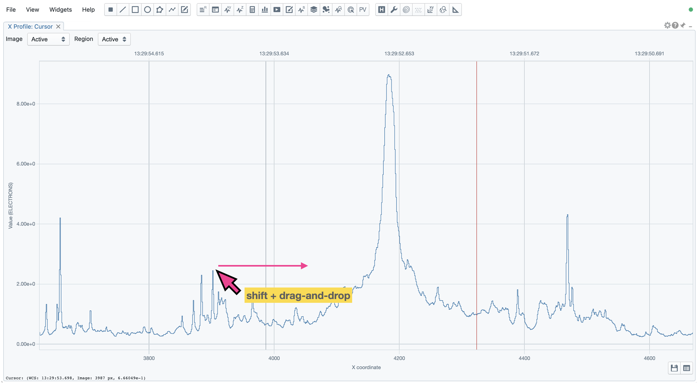
Horizontal pan
Hold the “shift” key, then drag-and-drop horizontally
Zooming a chart
A chart (profiles and histograms) can be zoomed in by scrolling up and zoomed out by scrolling down. Alternatively, horizontal zoom, vertical zoom, and box zoom are supported by drag-and-drop actions.
Panning a chart
A chart can be panned by holding the “shift” key and then applying drag-and-drop action. Panning in the x direction is supported only.
Resetting range
Double-clicking on the chart resets the plotting range.
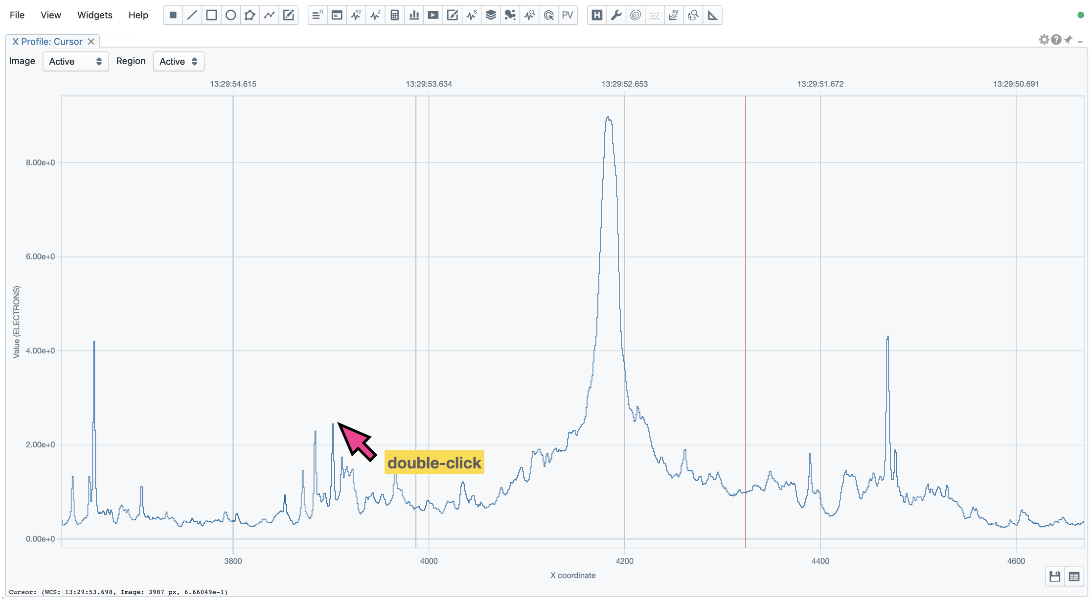
Configuring the layout#
Mouse actions, such as click or drag-and-drop can change the layout configuration. The drag-and-drop action is guided with a semi-transparent box. Various operations are described below. By mastering this section, you should be able to create, save, and restore custom layouts that fit your use cases.
Resizing a widget#
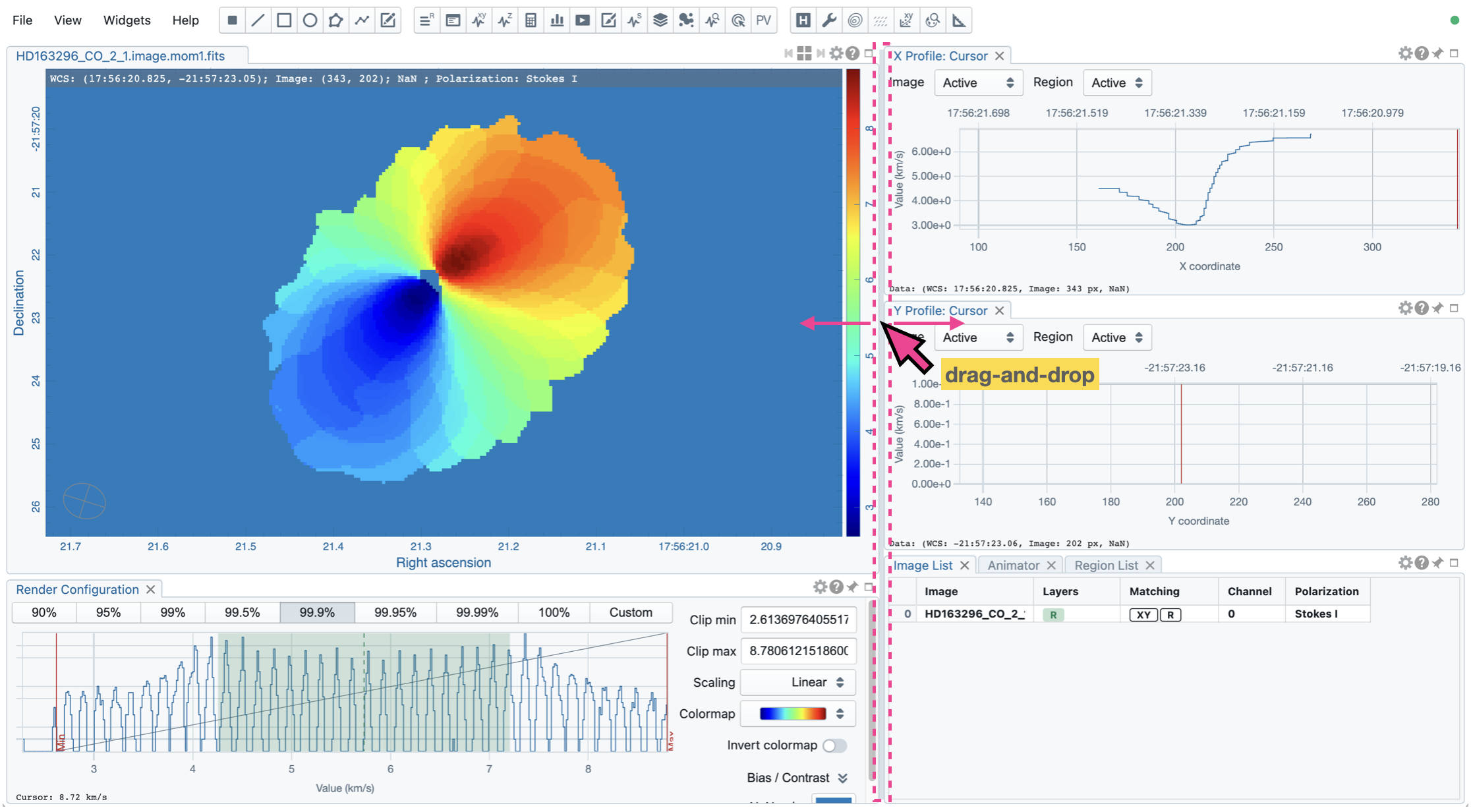
A widget can be resized by applying drag-and-drop action to its borders. After a panel is resized, adjacent panels are resized automatically to fit the new layout. The image size on the screen and the aspect ratio will be displayed for the Image Viewer after the widget size is changed.
Relocating a tab as a new docked widget#
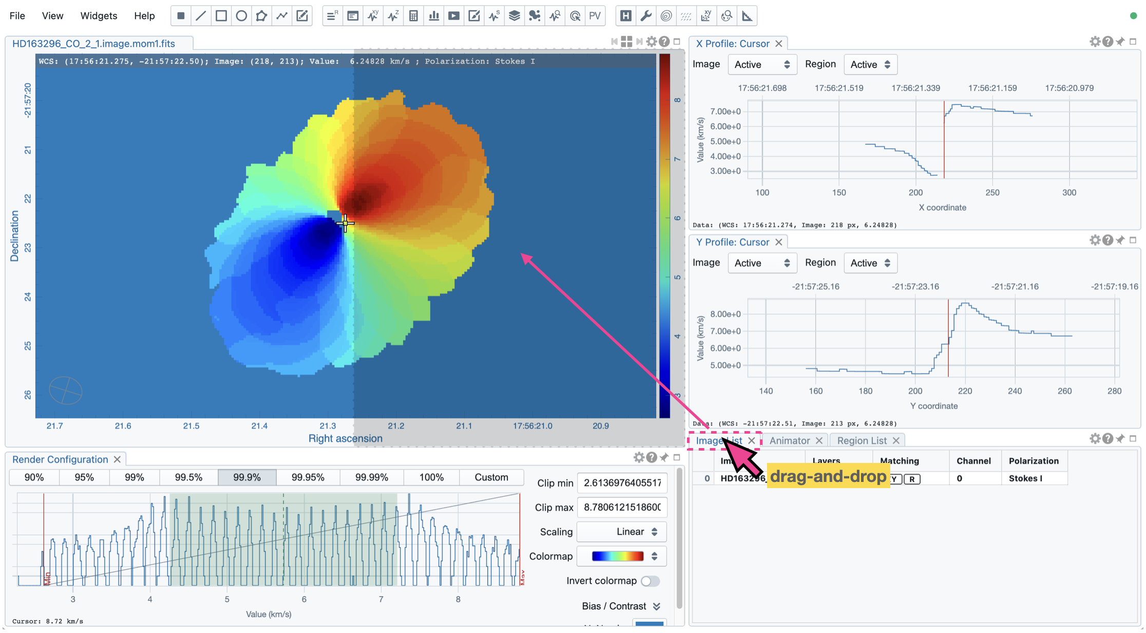
A tab (docked widget) can be detached and relocated by dragging its title to a desired location as a docked widget. The target location is visualized with a semi-transparent box, as shown in the example below.
Relocating a tab to share space with other docked widget#
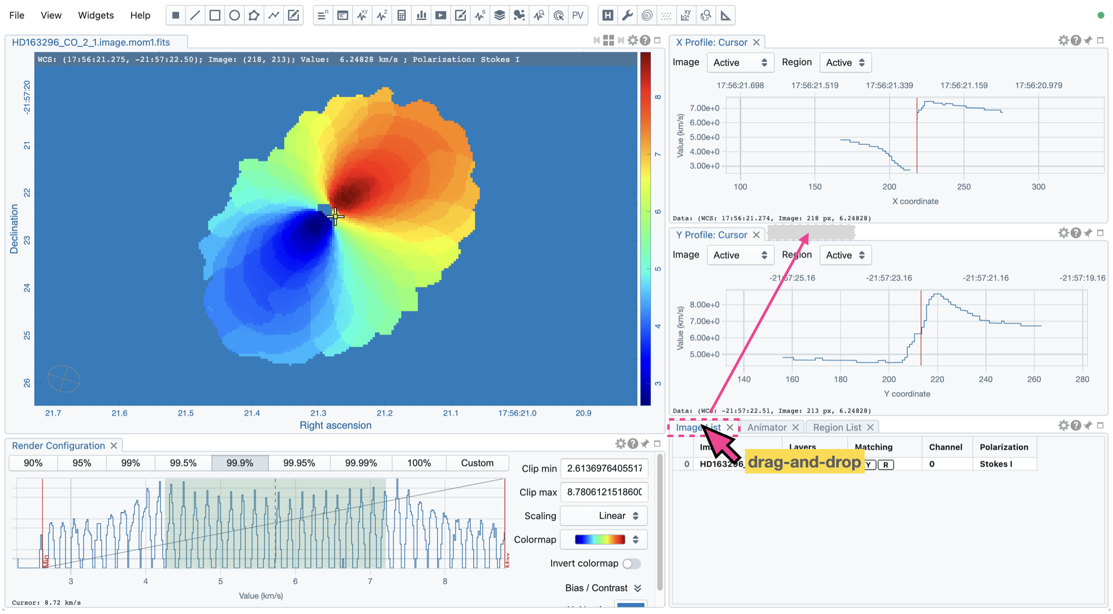
A tab (docked widget) can be moved to another existing docked widget to share space by dragging its title to the upper border of the target location, as shown in the example below.
Maximizing and restoring a widget#
By clicking the “maximize” button at the top-right corner of a docked widget, the widget (including all the other stacked widgets) will be maximized to the main browser window.
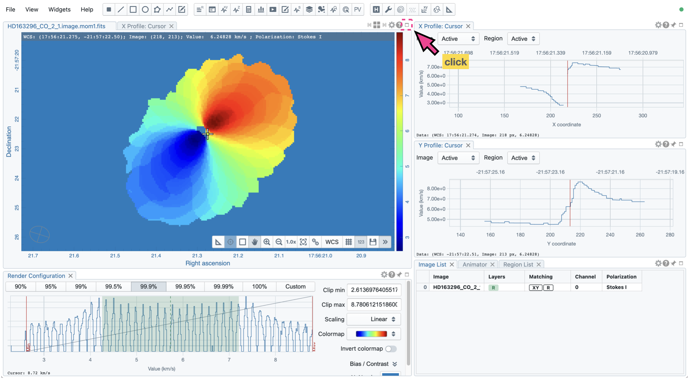
By clicking the “restore” button, the widget (and the other stacked widgets) will be restored to its original location.

Detaching and attaching a widget#
The active tab can be detached as a floating widget by clicking the “detach” (unpin) button at the top-right corner of a docked widget.
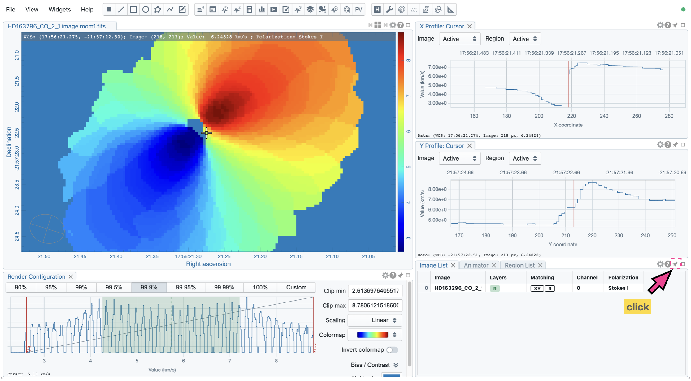
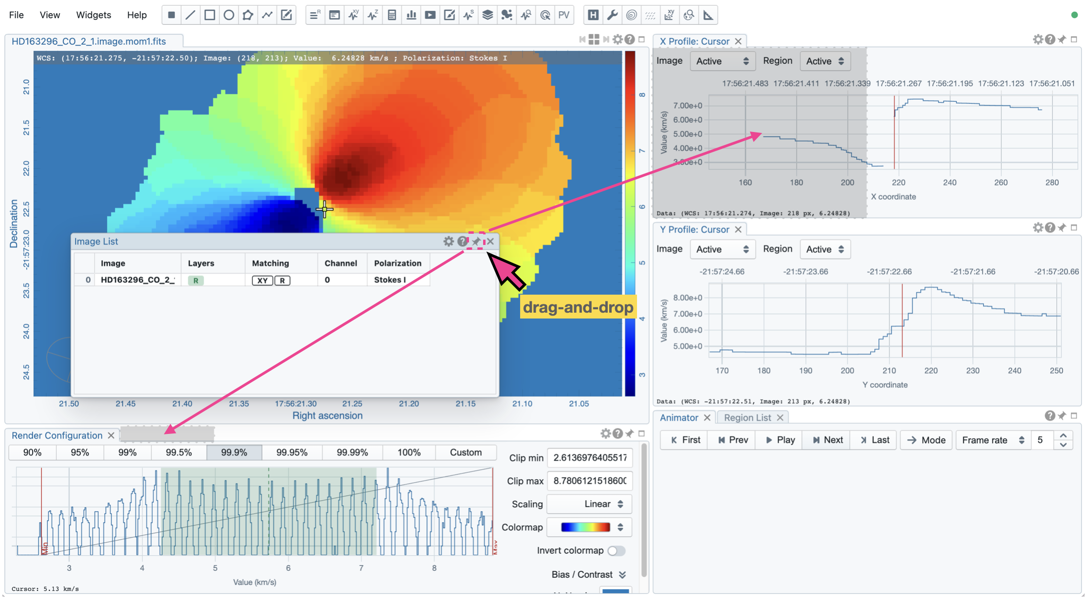
By dragging the “attach” (pin) button, a floating widget can be stacked with an existing docked widget or positioned as a docked widget.
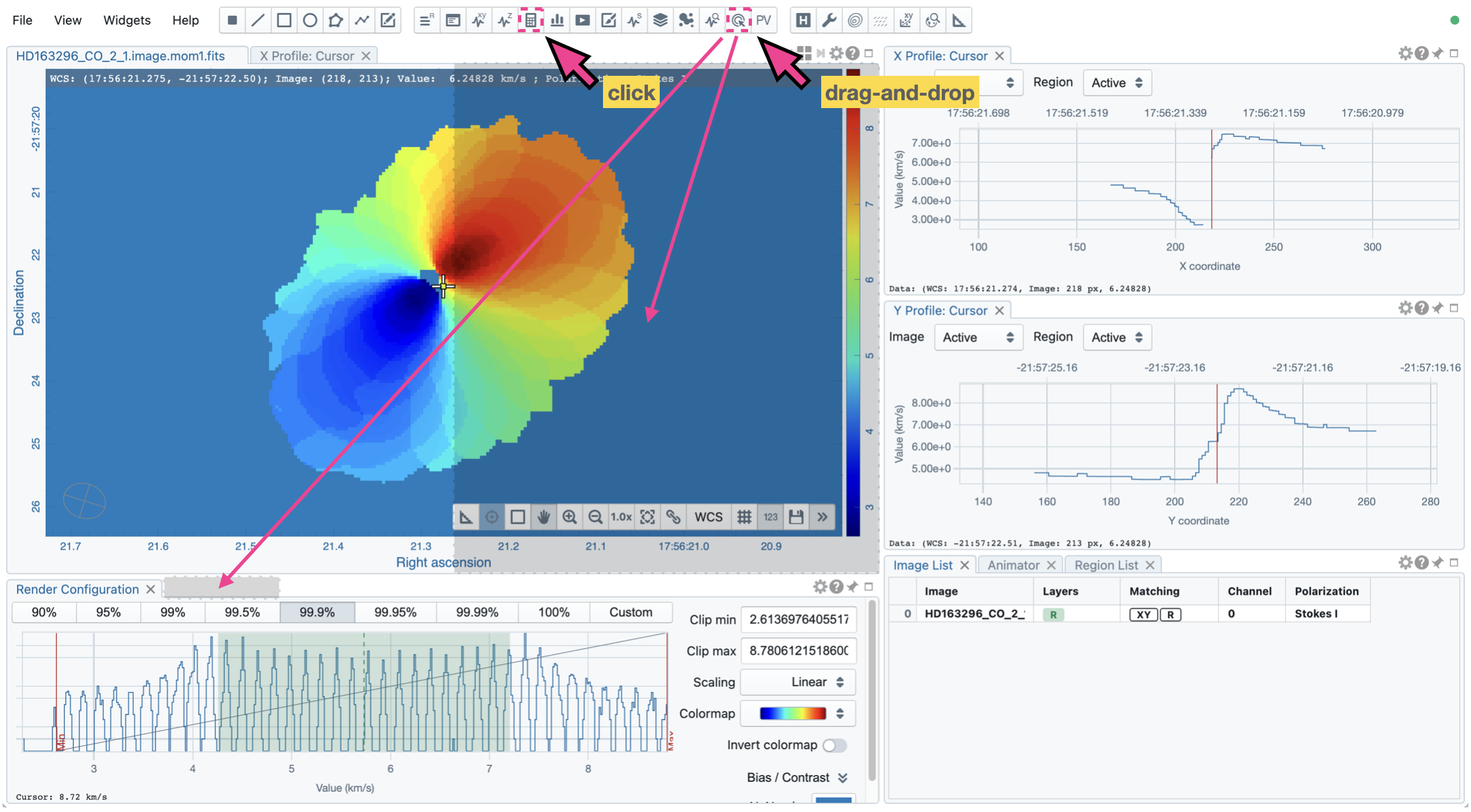
Creating a widget as a floating widget or as a docked widget#
A widget can be activated as a floating widget by clicking the desired widget button from the widget bar. Alternatively, a widget can be activated as a docked widget by dragging the desired widget button from the widget bar directly to a desired location.
Making the image viewer as a popout browser window#
This is a new feature introduced in CARTA v6.0. The Image Viewer can be popped out as a new browser window by clicking the “popout” button at the top-right corner of the Image Viewer. The popout window can be resized and moved freely just like a regular browser window. The popout window can be closed by clicking the “close” button of the browser window and the Image Viewer will be restored to the main browser window.
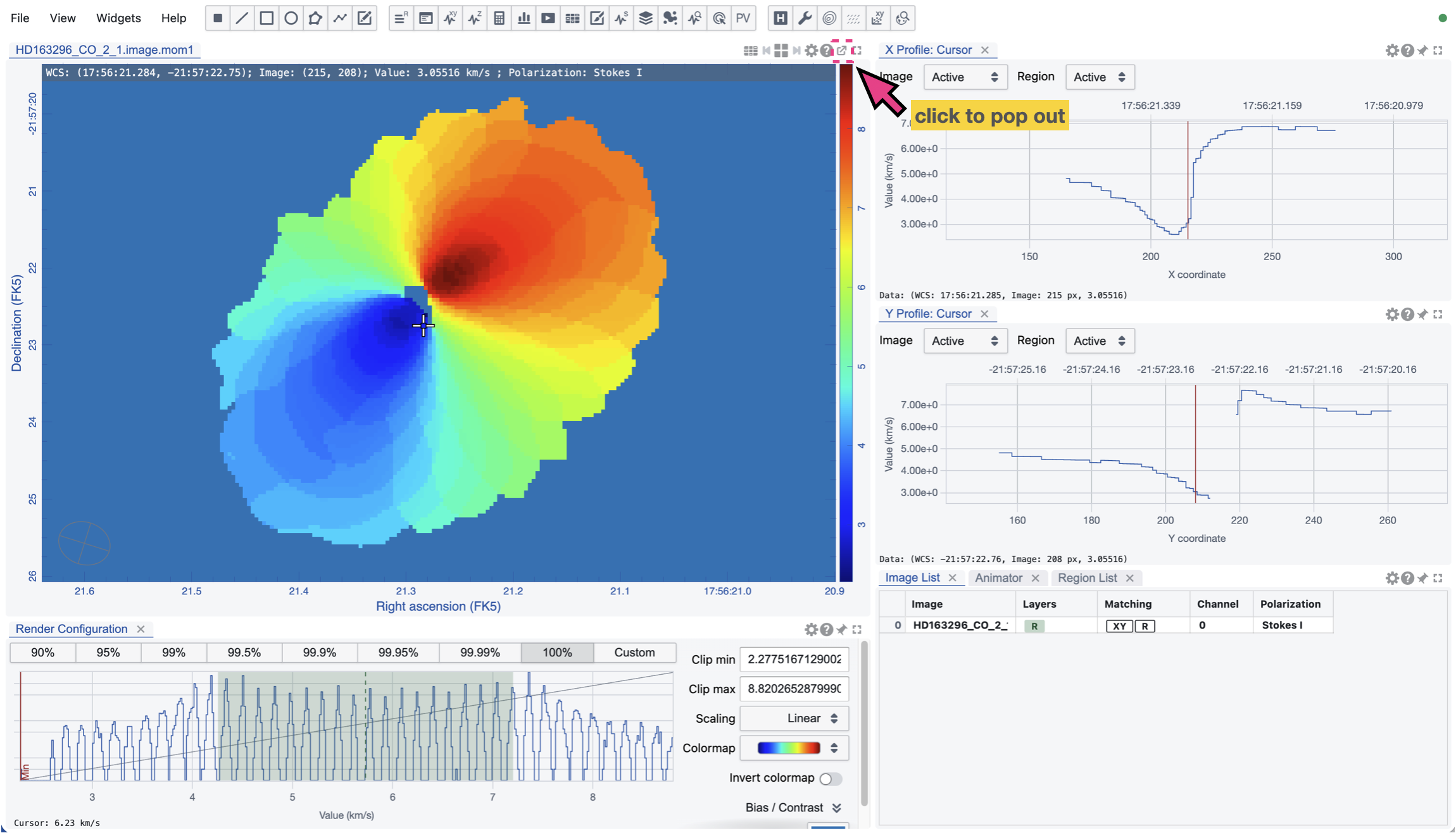
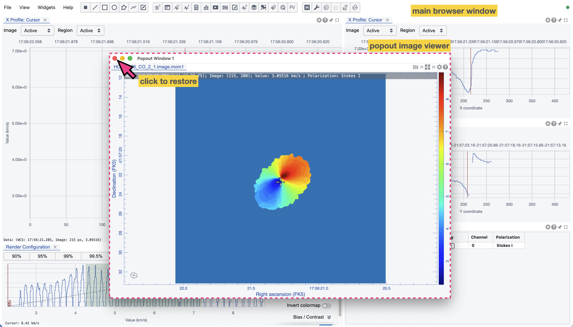
The best use case of this feature is to use a second monitor to display the Image Viewer while keeping the main browser window for other widgets, or vice verse. If you are using an extra-wide screen monitor or a regular monitor, it is still recommended to use a single browser window to display the Image Viewer and other widgets and utilize the layout management feature to configure the layout. This provides a seamless user experience when you switch focus between the Image Viewer and other widgets. When the Image Viewer is popped out as a new browser window, it is just like a regular browser window managed by the operating system. You will need to activate the browser window with an extra mouse click, with a keyboard shortcut, or enabling auto-focus on mouse hover before interacting with the content.
Light and dark themes#
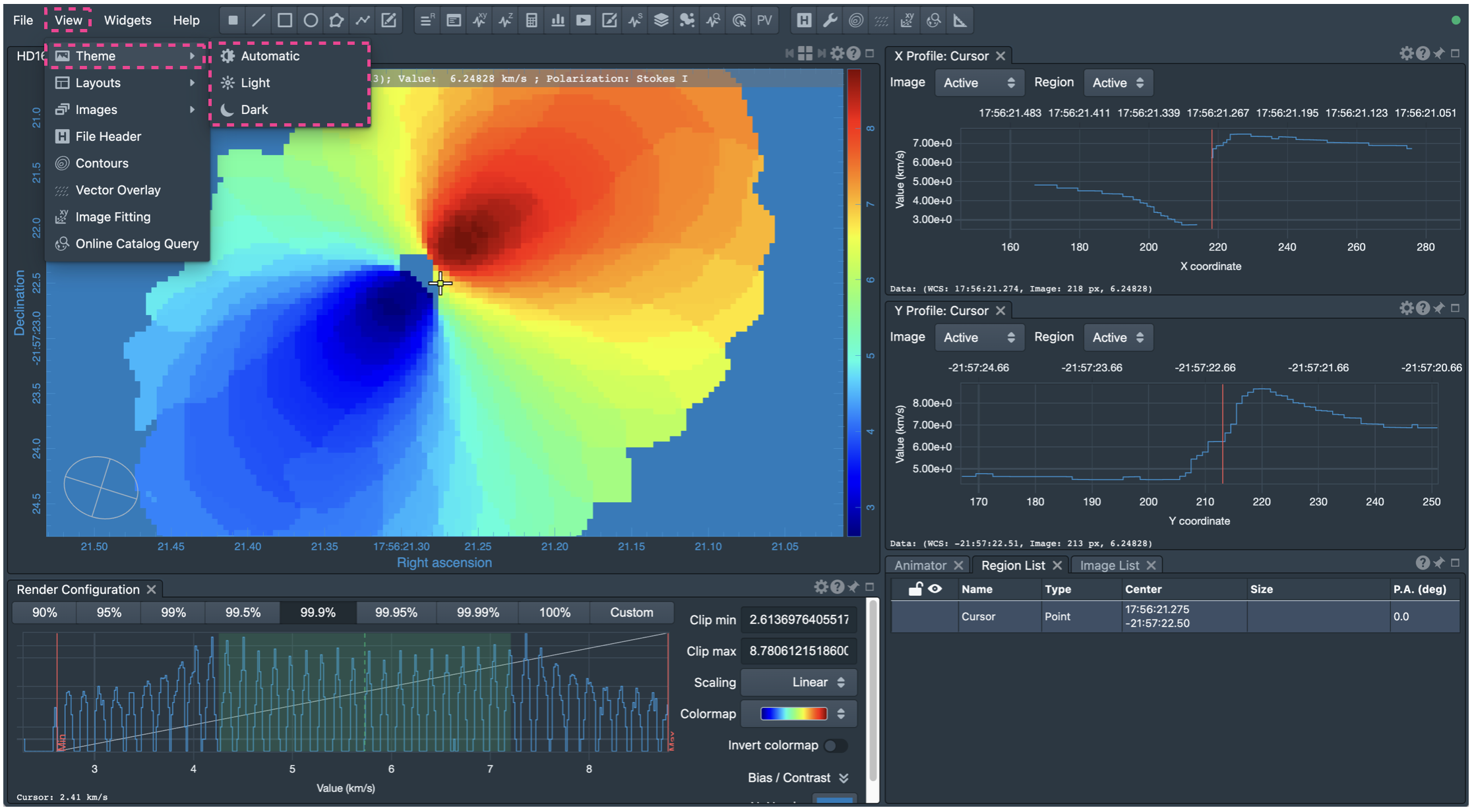
CARTA supports light and dark themes. The default theme is determined automatically from the operating system (if applicable). The theme can be changed using the menu “View” -> “Theme”, or the shortcut “shift” + “D”.
Save and restore layout#
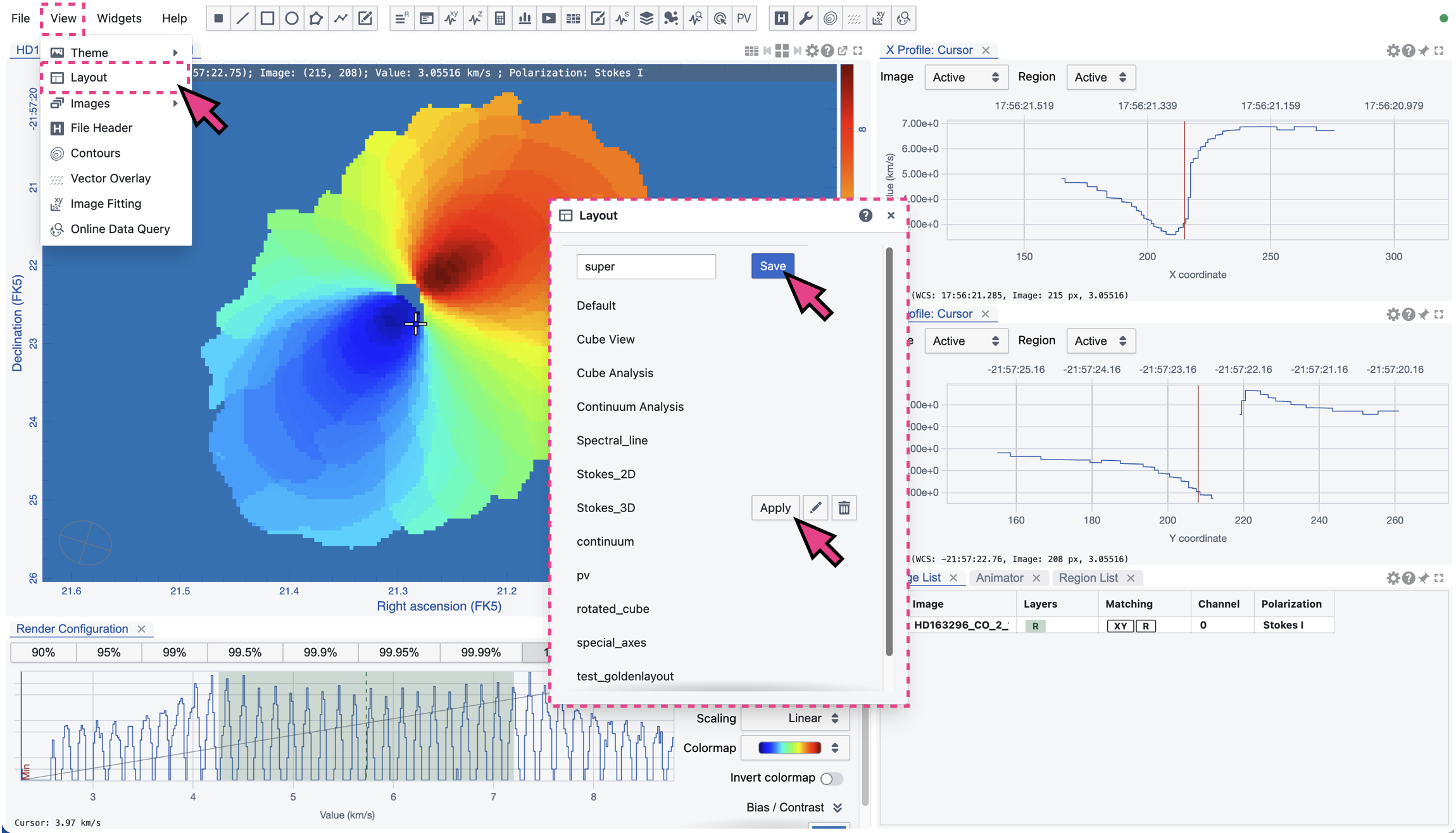
CARTA allows you to save the current layout as a custom layout. The saved layout can be restored later. To save or restore a layout, use the menu “View” -> “Layout”. For more information about layout management and dynamic layout, please refer to the section Layout.
Controls and shortcuts#
CARTA supports keyboard shortcuts to enable specific actions without using a mouse. A summary is accessible via the menu “Help” -> “Controls and Shortcuts”, or the shortcut “shift” + “?”. The shortcuts are slightly different depending on the operating system. The table below summarizes the shortcuts for each operating system.
Control |
macOS |
Linux |
|---|---|---|
Help |
||
Controls and shortcuts |
shift + ? |
shift + ? |
Navigation |
||
Pan image (two modes) |
drag-and-drop (default) / click |
drag-and-drop (default) / click |
Pan image (inside region) |
command + click / middle-click |
ctrl + click / middle-click |
Zoom image |
mouse wheel |
mouse wheel |
Regions |
||
Region properties |
double-click |
double-click |
Delete selected region |
del / backspace |
del / backspace |
Toggle region creation mode |
C |
C |
Deselect region |
esc |
esc |
Cancel region creation |
esc |
esc |
Switch region creation mode |
command + drag-and-drop |
ctrl + drag-and-drop |
Symmetric region creation |
shift + drag-and-drop |
shift + drag-and-drop |
Toggle current region lock |
L |
L |
Unlock all regions |
shift + L |
shift + L |
Move region (default step) |
arrow keys |
arrow keys |
Move region (coarse step) |
shift + arrow keys |
shift + arrow keys |
Move region (fine step) |
option + arrow keys |
alt + arrow keys |
Copy and paste region |
command + C / command + V |
ctrl + C / ctrl + V |
Multi-select regions |
command / ctrl + click |
ctrl + click |
Multi-select regions |
shift + click-and-drag |
shift + click-and-drag |
Toggle control point editing |
enter |
enter |
Deselect control point |
esc |
esc |
Cycle through control points |
tab or shift + tab |
tab or shift + tab |
Modify control point |
arrow keys |
arrow keys |
Modify control point (coarse) |
shift + arrow keys |
shift + arrow keys |
Modify control point (fine) |
option + arrow keys |
alt + arrow keys |
Appearance |
||
Toggle light/dark theme |
shift + D |
shift + D |
Cursor |
||
Freeze/unfreeze cursor |
F |
F |
Mirror cursor on multipanel view |
G |
G |
File controls |
||
Open image |
alt + O |
alt + O |
Append image |
alt + L |
alt + L |
Close image |
alt + W |
alt + W |
Save image |
alt + S |
alt + S |
Export image |
alt + E |
alt + E |
Import catalog |
alt + C |
alt + C |
Frame controls |
||
Next frame |
alt + ] |
alt + ] |
Previous frame |
alt + [ |
alt + [ |
Next channel |
alt + up |
alt + up |
Previous channel |
alt + down |
alt + down |
Next Stokes / polarization |
alt + shift + up |
alt + shift + up |
Previous Stokes / polarization |
alt + shift + down |
alt + shift + down |