
Contour rendering#
In addition to raster rendering, CARTA supports contour rendering as well. A contour image layer can be created on the same raster image or on a different raster image with world coordinates matched. The contour generation process is achieved with the Contour Configuration Dialog, which can be launched via the dialog bar.
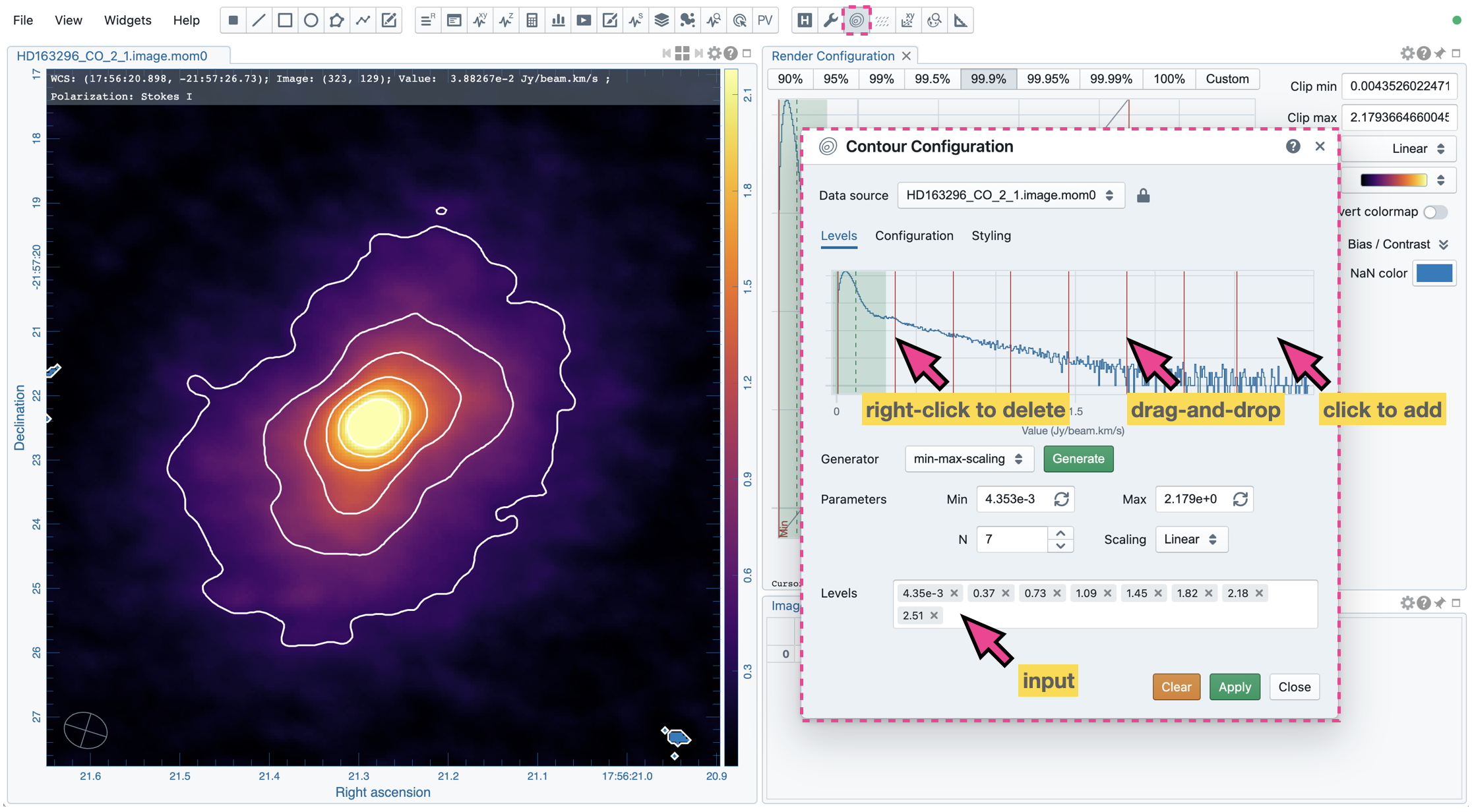
The Data source dropdown menu is used to select the input data for contour calculations. The lock button next to the dropdown menu is used to synchronize the displayed image in the Image Viewer with the selected data source. If the state is unlocked, changing the data source will not change the displayed image in the Image Viewer.
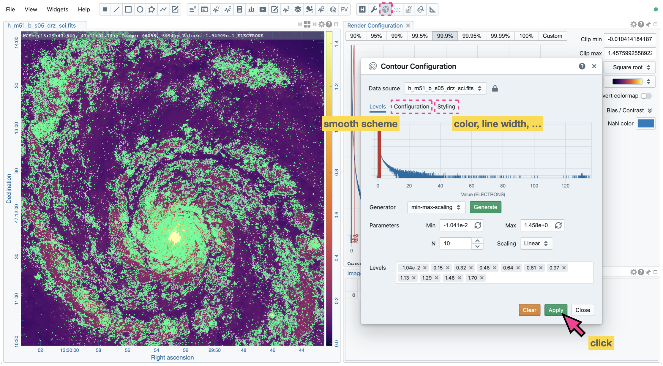
The Contour Configuration Dialog consists of three tabs: “Levels”, “Configuration”, and “Styling”. The “Levels” tab is used to define contour levels, the “Configuration” tab is used to define the contour smoothing scheme, and the “Styling” tab is used to define the appearance of contours.
The contour image is rendered on the client side using WebGL2, which allows for fast rendering of large contour images. The contour vertices are calculated on the server side and sent to the client for rendering. The contour rendering process is incremental, meaning that the contours will be drawn as soon as the vertices are available, allowing for a visualization of the contour generation process. This is particularly useful for large datasets or fine contour levels where the contour generation can take a long time.
Note
The contour rendering layer in the Image Viewer Widget may be hidden by clicking the “C” button in the Layers column of the Image List widget. When the contour layer of a given image is hidden, the same contour layer on all the other spatially matched images will also be hidden.
Reference steps to create contours#
You can follow the steps to generate a contour image:
Define contour levels. There are several ways to define a set of contour levels to be calculated on the server side:
by typing in individual levels in the “Levels” field manually
by using the “Generator” to compute a series of levels
by clicking directly on the histogram plot to create levels (right-click on an existing level to remove)
Note that the “Levels” field is editable even if the level generator has generated a set of levels.
(optional) Define a smooth scheme and a kernel size in the “Configuration” tab. The default is Gaussian smooth with a kernel size of 4 by 4 pixels.
(optional) Define the appearance of contours to be rendered on the client side in the “Styling” tab. The appearance of contours can be modified after a set of contours has been rendered at the client side without triggering new contour calculations on the server side. This is the advantage of utilizing WebGL2 on the client side.
After defining a set of levels, click the “Apply”” button to view the contour image. The contour image will be rendered incrementally if there are numerous contour vertices.
Matching contour images to raster images#
In the figure above, a contour image is rendered on top of the same raster image. Suppose you want to plot a contour image on top of another raster image (e.g., velocity field as contour, integrated intensity image as raster). In that case, you need to enable WCS matching of the two raster images first (see Image matching). Then, you can generate a contour image just like the example below. The contour images will be visible on all the images that are matched to the spatial reference image in world coordinates, including the spatial reference image itself.
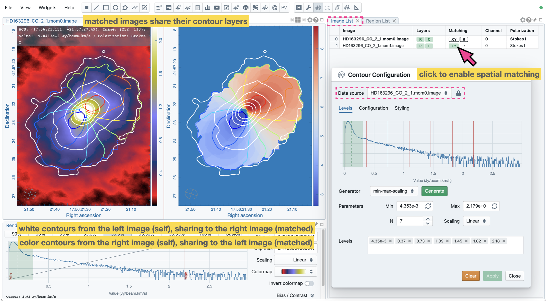
If multiple images are loaded in the append mode, you may use the “Data Source” dropdown menu to select an image as the input data for contour calculations. If the state of the “lock” button is locked, the Image Viewer will show the selected image as a raster image, and the image slider in the Animator Widget will be updated to the selected image too. To turn off this synchronization, click the “lock” button to set the state to unlocked.
Contour level generators#
CARTA provides four different level generators to assist you in defining a set of contour levels.
“start-step-multiplier”
A set of “N” levels will be computed from “Start” with a (variable) “Step” and a “Multiplier”. For example, if start = 1.0, step = 0.1, N = 5, and multiplier = 2, five levels will be generated as “1.0, 1.1, 1.3, 1.7, 2.5”. The function of the multiplier is to make the step increase for each next new level. Default parameters derived from the full image statistics (per-channel) are:
start: mean + 5 * standard deviation
step: 4 * standard deviation
N: 5
multiplier: 1
“min-max-scaling”
A set of “N” levels will be calculated between “Min” and “Max” based on the “Scaling” function. For example, if min = 2, max = 10, N = 5, scaling = “linear”, five levels will be generated as “2, 4, 6, 8, 10”. Default parameters derived from the full image statistics (per-channel) are:
min: lower bound of 99.9% clip
max: upper bound of 99.9% clip
N: 5
scaling: “linear”
“percentages-ref.value”
A set of “N” levels will be derived as the percentages (”Lower(%)” and “Upper(%)”) of the “Reference” in linear spacing. For example, if reference = 1.0, N = 5, lower(%) = 20, upper(%) = 100, five levels will be generated as “0.2, 0.4, 0.6, 0.8, 1.0”.
reference: upper 99.9% clip
N: 5
lower(%): 20
upper(%): 100
“mean-sigma-list”
A set of “N” levels will be generated as “Mean” plus multiples of “Sigma” based on the “Sigma list”. For example, if mean = 1, sigma = 0.1, and sigma list = [-5, 5, 10, 15, 20], five levels will be generated as “0.5, 1.5, 2.0, 2.5, 3.0”. Default parameters derived from the full image statistics (per-channel) are:
mean: full image mean value
sigma: full image standard deviation
sigma list: [-5, 5, 9, 13, 17]
Smoothing modes#
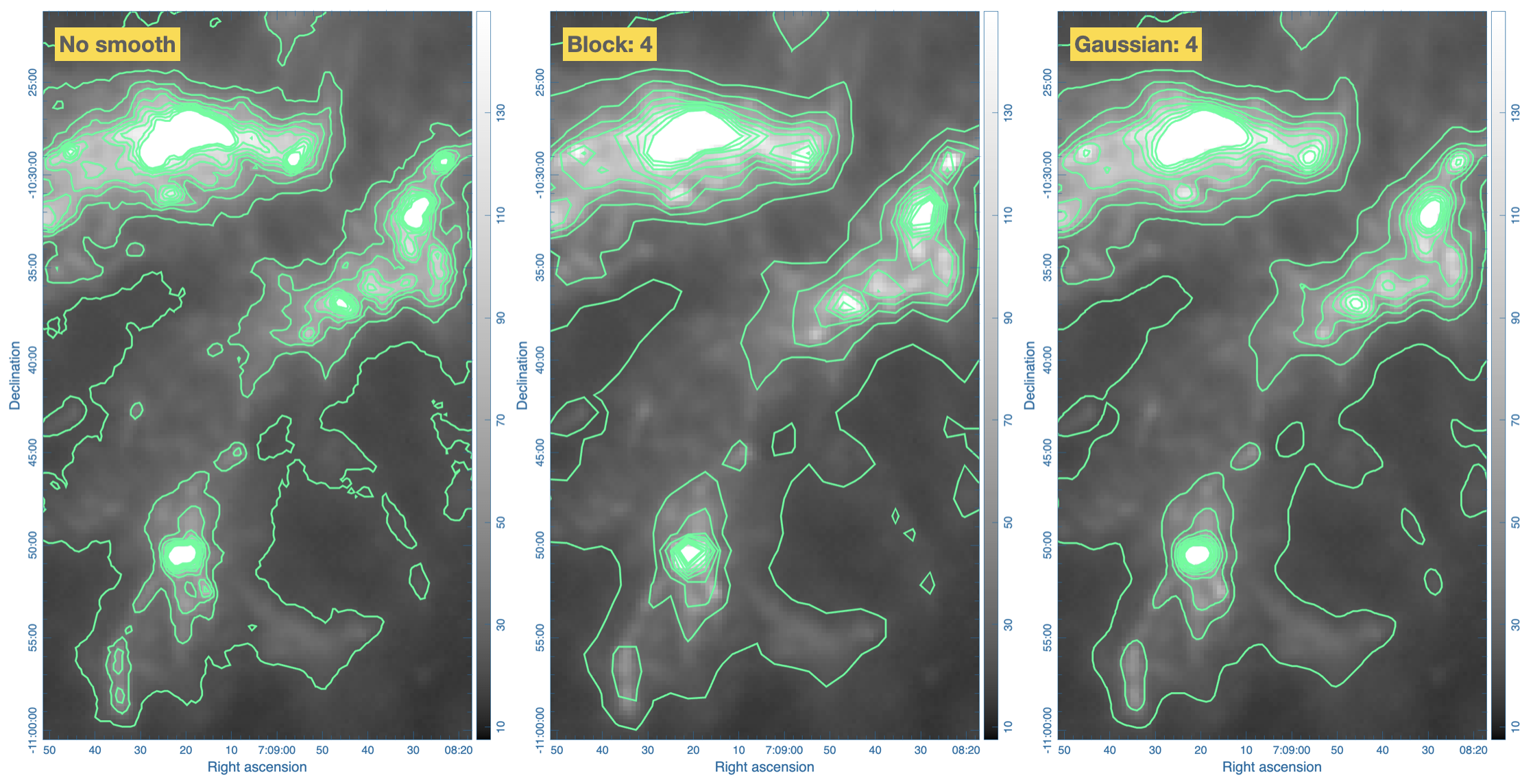
CARTA provides three different contour smoothing methods, including “no smooth”, “Gaussian smooth”, and “block smooth”, in the “Configuration” tab. The kernel for smoothing is in N by N pixels. The default is to apply “Gaussian smooth” with 4 pixels by 4 pixels as the kernel size. You may choose a different smooth method and kernel size depending on science cases.
Styling contours#
The appearance of contours can be customized in the “Styling” tab. For example, you may use the options to plot contours like below. Iso-velocity contours are rendered in different colors to represent the Doppler shifts of the source kinematics.
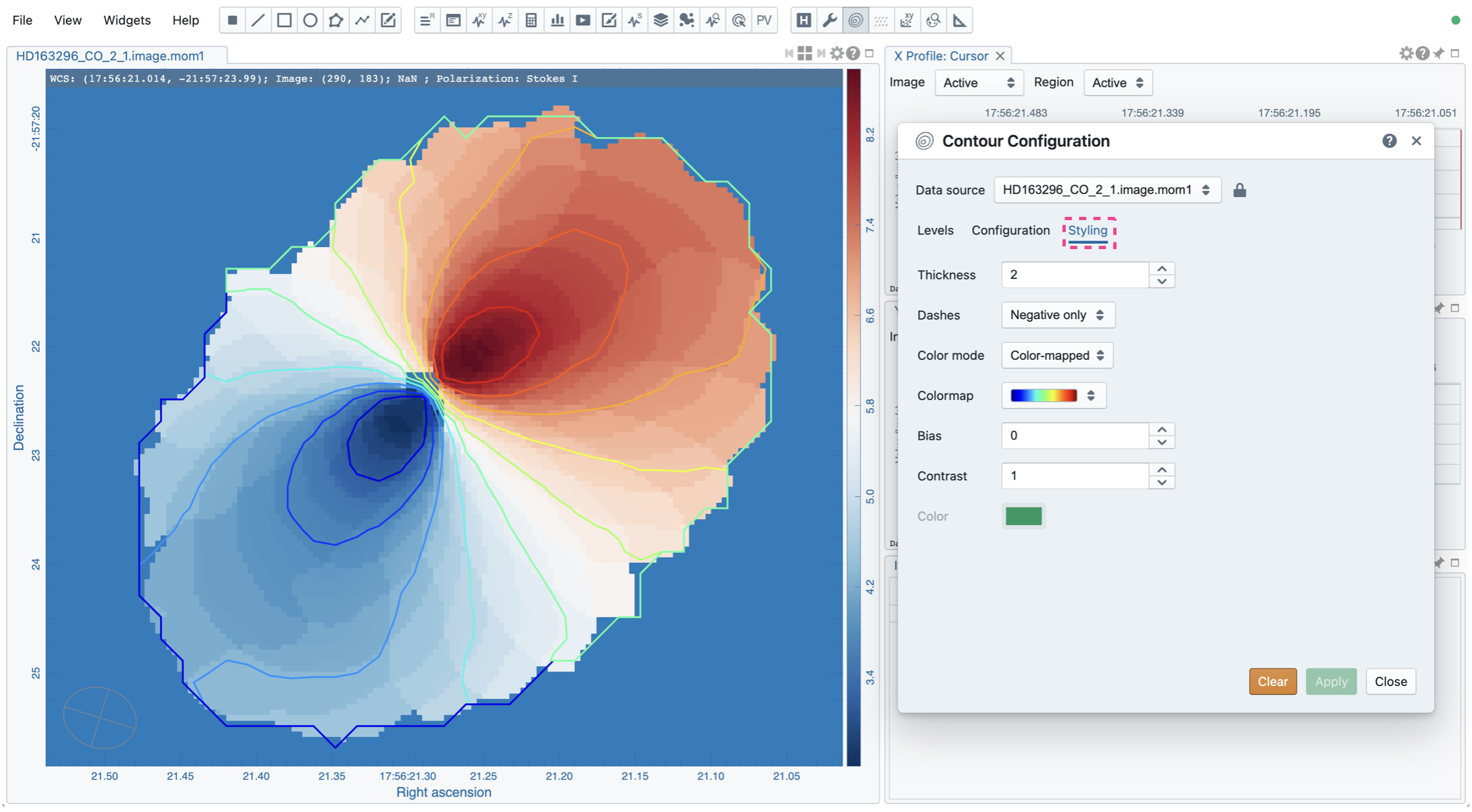
Changing the contour styling will not trigger a new contour calculation on the server side, which is the advantage of using WebGL2 for client-side contour rendering. You can change the contour styling anytime after the contours have been rendered and see the results immediately.