File browser#
Note
Image files#
The File Browser, accessible via the menu “File” -> “Open Image” or the menu “File” -> “Append Image”, provides a list of images and their information supported by CARTA. The supported image formats are:
CASA format
HDF5 format (IDIA schema, see HDF5 (IDIA schema) image support)
FITS format
MIRIAD format
Only images that match these formats will be shown in the file list by default. If you usually work with directories containing lots of files, you may switch to a different file list generation mode via “File” -> “Preferences” -> “Global” -> “File List”. The performance of the file list generation can be improved by just using the file extension as the parser or by simply listing all files without parsing the image type.
When an image is selected, a summary of image properties is provided on the right-hand side of the dialog. The full image header is available in the second tab. To view an image, click the “Load” button at the bottom-right corner. You can also double-click an image to load it directly. To view a new image and close all the loaded images, use the “File” -> “Open Image” -> “Load” button. To view a new image without closing all the loaded images, use the “File” -> “Append Image” -> “Append” button.

If multiple images are required to perform joint visualization and analysis (e.g., CO 2-1, 13CO 2-1, and C18O 2-1), you can select multiple files in the file list with “shift+click”/”command+click” (macOS) or “shift+click”/”ctrl+click” (Linux) and load or append them all at once.

You can search for files and sub-directories using the filter field located at the bottom of the File Browser. Three different methods are supported:
Fuzzy search: free typing
Unix pattern: e.g.,
*.fitsRegular expression: e.g.,
colou?r
The File Browser remembers the last path where an image was opened within one CARTA session, and the path is displayed (as breadcrumbs) at the top of the File Browser. Therefore, when the File Browser is re-opened to load other images, a file list will be displayed at the path where the previous image was loaded. CARTA can also remember the last path for a new CARTA session via “File” -> “Preferences” -> “Global” -> “Save last used directory”.
You can use the breadcrumbs to navigate to one of the parent directories or click the home button to directly navigate to the base (i.e., initial) directory. Alternatively, you can use the pencil button and enter a path (with respect to the top level folder which is specified with the --top_level_folder flag when starting the carta_backend) directly to switch directories. You can click the reload button to get an updated file list from the server side.

Note
For the CARTA deployed in the “Site Deployment Mode”, the server administrator can limit the global directory access through the --top_level_folder flag when a CARTA backend service is initialized.
exec carta_backend /scratch/images/Orion --top_level_folder /scratch/images
In the above example, you will see a list of images at the directory “/scratch/images/Orion” when you access the File Browser Dialog for the first time in a new session. You can navigate to any other folders inside “/scratch/images/Orion”. You will navigate to the directory “/scratch/images/Orion” directly by clicking the home button. You can also navigate one level up to “/scratch/images”, but not beyond that (neither “/scratch” nor “/”) as limited by the --top_level_folder flag.
An image can be closed via “File” -> “Close Image”. The active image (the image in the single-panel view or the image highlighted with a red box in the multi-panel view) will be closed. Alternatively, you can close an image via the context menu (right-click) in the Image List Widget. Note that if the image being closed is a WCS reference image, any other matched images to this reference image will be unmatched. Therefore, they will be just like individual images.
Tip
An image may be opened directly using a modified URL. For example, if you want to open an image file “/home/acdc/CARTA/Images/jet.fits”, you can append
&folder=/home/acdc/CARTA/Images&file=jet.fits
or
&file=/home/acdc/CARTA/Images/jet.fits
to the end of the URL (e.g., http://192.168.0.128:3002/?token=E1A26527-8226-4FD5-8369-2FCD00BACEE0). In this example the full URL is
http://192.168.0.128:3002/?token=E1A26527-8226-4FD5-8369-2FCD00BACEE0&folder=/home/acdc/CARTA/Images&file=jet.fits
or
http://192.168.0.128:3002/?token=E1A26527-8226-4FD5-8369-2FCD00BACEE0&file=/home/acdc/CARTA/Images/jet.fits
Please note that it is necessary to supply a full path. Tilde (~), as your home directory, is not allowed.
Note
CARTA image loading performance
The per-channel rendering approach helps to improve the performance of loading an image. Traditionally, when an image is loaded, the minimum and maximum of the entire image (cube) are computed first before image rendering. This becomes a severe performance issue if the image (cube) size is huge (more than a few tens to hundreds of GB). In addition, applying the global minimum and maximum to render a raster image usually (if not often) results in a poorly rendered image if the dynamic range is high. Then, you will need to re-render the image repeatedly with refined boundary values. Re-rendering such a large image repeatedly with CPUs further deduces user experiences.
CARTA improves the image viewing experience by adopting GPU-accelerated rendering techniques in the web browser environment. In addition, CARTA only renders an image with sufficient image resolution (image tiles with a proper down-sampling factor) for your screen. This combination results in a scalable and high-performance remote Image Viewer. The total file size is no longer a bottleneck. The determinative factors are 1) image size in x and y dimensions, 2) internet bandwidth, and 3) storage I/O performance, instead. For a laptop with 8 GB of RAM, the largest image it can load without memory swapping is about 40000 pixels by 40000 pixels (assuming most of the RAM is free before loading the image).
The approximated RAM usage for loading images with various spatial sizes is summarized below.
Image size (x, y) [pixel] |
RAM usage |
|---|---|
512 |
1 MB |
1024 |
4 MB |
2048 |
16 MB |
4096 |
64 MB |
8192 |
256 MB |
16384 |
1 GB |
32768 |
4 GB |
65536 |
16 GB |
HDF5 (IDIA schema) image support#
Beside the CASA image format, the FITS format, and the MIRIAD format, CARTA also supports images in the HDF5 format following the IDIA schema. The IDIA schema is designed to ensure efficient image visualization is retained even with huge image cubes (hundreds of GB to a few TB). The HDF5 image file contains extra data to skip or speed up expensive computations, such as per-cube histogram, spectral profile, etc. Below is a summary of the content included in an HDF5 image:
XYZW dataset (spatial-spatial-spectral-Stokes): similar to the FITS format
ZYXW dataset: rotated dataset
Per-channel statistics: basic statistics of the XY plane
Per-cube statistics: basic statistics of the XYZ cube
Per-channel histogram: histogram of the pixel values of the XY plane
Per-cube histogram: histogram of the XYZ cube
Per-channel mip map: downsampled image tiles
The CARTA development team provides a FITS-to-HDF5 converter for you to convert a FITS image to the HDF5 (IDIA schema) format. You can refer to Installation of fits2idia (converting FITS to HDF5-IDIA) on how to install fits2idia program on your platform.
The fits2idia usage is the following:
IDIA FITS to HDF5 converter version 0.1.15 using IDIA schema version 0.3
Usage: fits2idia [-o output_filename] [-s] [-p] [-m] input_filename

Options:
-o   Output filename
-s   Use slower but less memory-intensive method (enable if memory allocation fails)
-p   Print progress output (by default the program is silent)
-m   Report predicted memory usage and exit without performing the conversion
-q   Suppress all non-error output. Deprecated; this is now the default.
Note
Currently the per-plane beam table is not supported in the HDF5 (IDIA schema) format.
Loading a Position-Velocity (PV) image#
You can load a position-velocity (PV) image in CARTA. When the image header has sufficient information for the spectral conversion of the “V” axis (e.g., velocity <-> frequency), you can apply the conversion via the “Conversion” tab of the Image Viewer Settings Dialog (the “cog” button at the top-right corner of the Image Viewer Widget).

Loading images with the Lattice Expression Language (LEL)#
CARTA supports loading images via the Lattice Expression Language (LEL) interface. To enable this feature, click the “Filter” dropdown menu in the File Browser and switch to the “Image arithmetic” mode. Please refer to the Lattice Expression Language for detailed usages.

With the LEL interface, you can apply arithmetic on images and load the result as an image in CARTA. For example, with the expression
"line_plus_continuum.fits" - "continuum.fits"
a “line only” image will be computed and loaded in CARTA.
When the LEL interface is enabled, you can either manually enter the expression in the expression field or use a mouse click to auto-complete an image file name to speed up the process.
If you need to save the image computed via the LEL interface, go to the “File” menu and select “Save Image”.
Loading a complex-value image#
A complex-value CASA image is supported in CARTA. When a CASA image is detected as complex-value, the “Load as” button includes the following components:
Amplitude
Phase
Real
Imaginary
as loading options. You can select a desired component to load or append.

If you want to save a component (e.g., Amplitude) as a new image file with the float data type, go to the “File” menu and select “Save Image”.
Loading an axes-swapped image cube#
CARTA supports a axes-swapped image cube. When such a cube is selected in the file list, the file information panel will show the labels of the axes in order. The first two axes will be used for rendering the XY plane in the Image Viewer. The Stokes axis (if there is any) will still be interpreted as a polarization axis. The third axis (excluding the Stokes axis, if there is any) will be interpreted as the Z axis for animation playback. In the following example, CARTA will render a FREQ-RA image in the Image Viewer. With the Animator Widget, you can trigger animation playback of the DEC axis (or the polarization axis, if there is any).

Warning
In v6.0, CARTA supports axes-swapped image cubes for image visualization only. Region analytics tools are not supported.
FITS image file association with the macOS Electron Desktop#
This is a new feature in the macOS Electron Desktop version of CARTA, starting from v6.0.
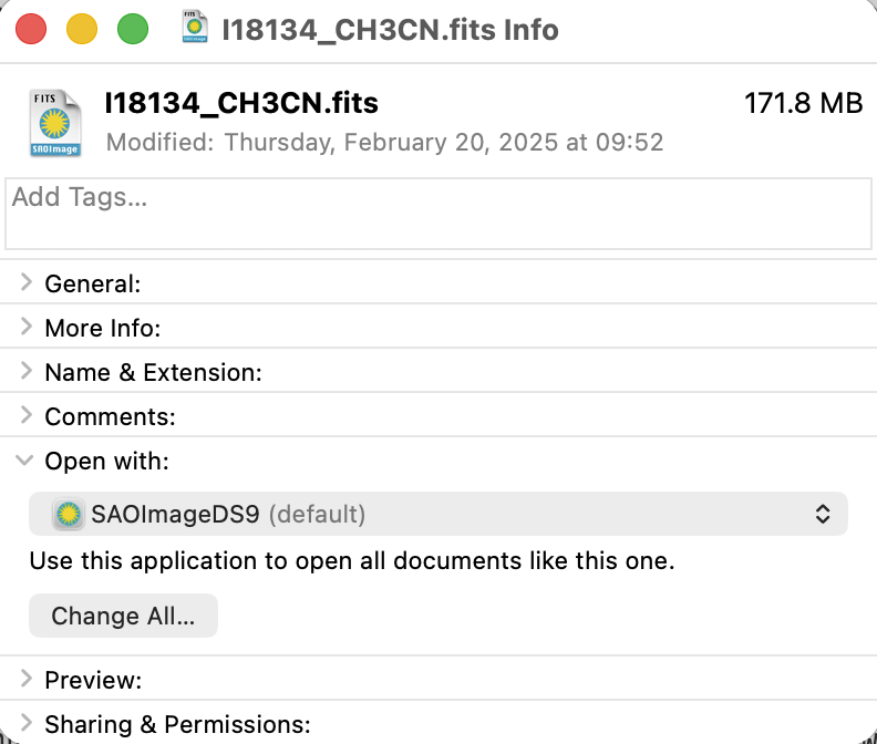
For users who have installed the macOS Electron Desktop version of CARTA, you can associate the FITS image file extension with the CARTA application by using the macOS context menu. To do this, right-click on a FITS image file in Finder, select “Get Info”, and then under the “Open with” section, choose CARTA from the dropdown menu. After that, click the “Change All…” button to apply this association to all FITS image files.
After the association is set up, you can double-click a FITS image file in Finder to open it in the CARTA Electron Desktop as a new session directly. You can also drag and drop a FITS image file or a set of FITS image files from Finder to the CARTA application icon in the Dock to open the image or images in CARTA. You may also drag and drop a FITS image file or a set of FITS image files from Finder to the CARTA application window to open or append the image or images in the current session of CARTA.
Stokes hypercube#
Suppose a set of individual Stokes images needs to be loaded into CARTA for data inspection with the Stokes Analysis Widget. In that case, you can multi-select individual Stokes images (e.g., image_I.fits, image_Q.fits, image_U.fits, and image_V.fits) in the file list with “shift+click”/”command+click” (macOS), or “shift+click”/”ctrl+click” (Linux), and load them with the “Load as hypercube”. A dialog will show up for you to confirm the identification (based on image headers or file names) of the Stokes parameters of the selected images. After clicking the “Load” button, the backend will form a hypercube from the selected images. Effectively, only one (virtual) image with multiple Stokes parameters is loaded in CARTA.

If you need to save a Stokes hypercube as an image file, go to the “File” menu and select “Save Image”.
Multi-color image blending#
CARTA supports a raster rendering mode by combining multiple images into one in the color space. This is an enhanced version of the traditional three-color (RGB) blending of astronomical images to create a pseudo-color image. In our implementation, multiple images with different image sizes and pixel sizes can be combined with various raster rendering configurations by taking advantage of the GPU power. The only requirement is selected images need to be matchable and do not have significant projection distortion in the image field. This feature serves as a unique tool for making publication-quality images, for example.
When multiple images are selected in the File Browser Dialog, a “Load with RGB blending” (two or three images) or a “Load with multi-color blending” (more than three images) will appear in the bottom-right corner. By clicking the button, the selected images will be loaded into CARTA with spatial matching enabled and a pre-defined raster rendering configuration for each image. Then the outcome raster image will be appended in the Image List widget and displayed in the Image Viewer. You can use the Raster Configuration Widget to perform detailed customization for each input image and for the multi-color blending image. See Multi-color image blending for more information.

The multi-color blending image cannot be saved as an image file (e.g., FITS). Instead, you will need to use the workspace feature (see Workspace for more information) to save the entire multi-color blending process as a snapshot for future useage. Use “File” -> “Save workspace” and use the popup dialog for saving. Use “File” -> “Open workspace” and the popup dialog to load a snapshot and restore the multi-color blending image.

Region files#
A region file in the CASA CRTF format or the ds9 reg format can be imported via “File -> “Import Regions”. When a region file is selected, its content is shown in the Region Information tab. All or a subset of regions can be exported as a region text file via “File” -> “Export Regions”. CASA and ds9 region text file definitions in world or image coordinates are supported. Note that regions can only be exported if appropriate write permissions are configured on your file system.
You can load multiple region files at once by selecting multiple region files with “ctrl/cmd+click” or “shift+click” in the file list, and then clicking the “Load region” button.

See Region of interest for more information.
Catalog files#
A catalog file in the FITS format or the VOTable format can be loaded and visualized as a table via “File” -> “Import Catalog”. When a catalog file is selected, its basic catalog properties are summarized in the Catalog Information tab on the right-hand side. Full catalog column header is shown in the Catalog Header tab.
You can load multiple catalog files at once by selecting multiple catalog files with “ctrl/cmd+click” or “shift+click” in the file list, and then clicking the Load catalog button.

See Catalog visualization for more information.