Image cube visualization

With v4.1.0, CARTA provides the following widgets and dialogs for image cube visualization:

• Widget

  • Image Viewer Widget: to view raster images and contour images

  • Render Configuration Widget: to configure how a raster image is rendered

  • Animator Widget: to navigate through different images, different channels, or different polarization components

  • Image List Widget: to configure image matching in world coordinates and the spectral domain

• Dialog

  • File Browser Dialog: to view image headers and to load or append an image

  • Contour Configuration Dialog: to configure how a contour image is computed and rendered

  • Vector Overlay Configuration Dialog: to configure how a vector overlay is computed and rendered

  • File Header Dialog: to view the image header

  • Image View Settings Dialog: to configure the appearance of an image in the Image Viewer

Server-side status and session resume

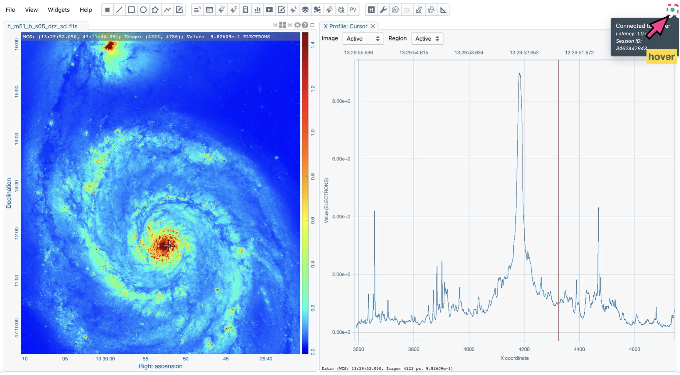
As CARTA is fundamentally a client-server application, it would be essential to know the status of the server side at the client side (i.e., your web browser). It is also helpful to know whether the standalone version runs normally. The server (i.e., the carta_backend) status is displayed as a circular icon in the top-right corner of the main browser window. The connection latency and a session ID can be seen by hovering over the icon. There are three kinds of status:

• Green: This means that the server side is connected successfully.

• Orange: This means that the initial connection to the server side was broken (e.g., unstable internet) but has been reconnected. You will be asked to resume the previous session or not.

• Red: This means that the server side is not accessible, either due to a broken internet or a backend crash. CARTA is not functional in this case.

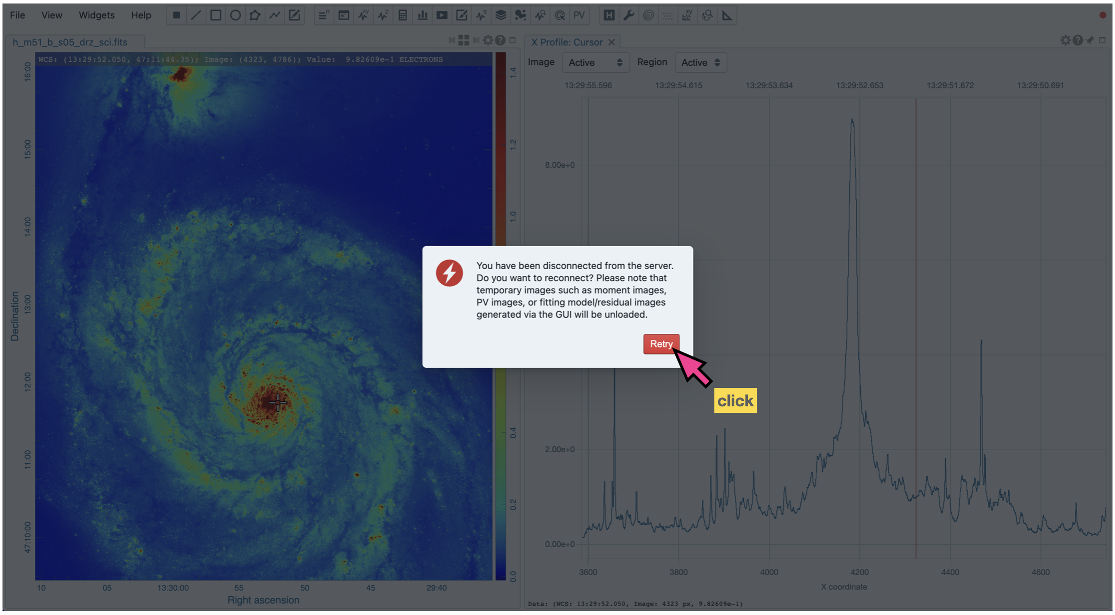
If CARTA behaves abnormally or stops responding, please check the server-side status icon and the connection latency. If it becomes red, the connection between the client and server sides is interrupted. At this point, CARTA is not functional. A prompt will be shown in the browser to ask you whether or not to resume the previous CARTA session. By clicking the “Retry” button, CARTA will try to resume the previous session if possible. If you choose not to resume the previous session, please reload CARTA to establish a new session.

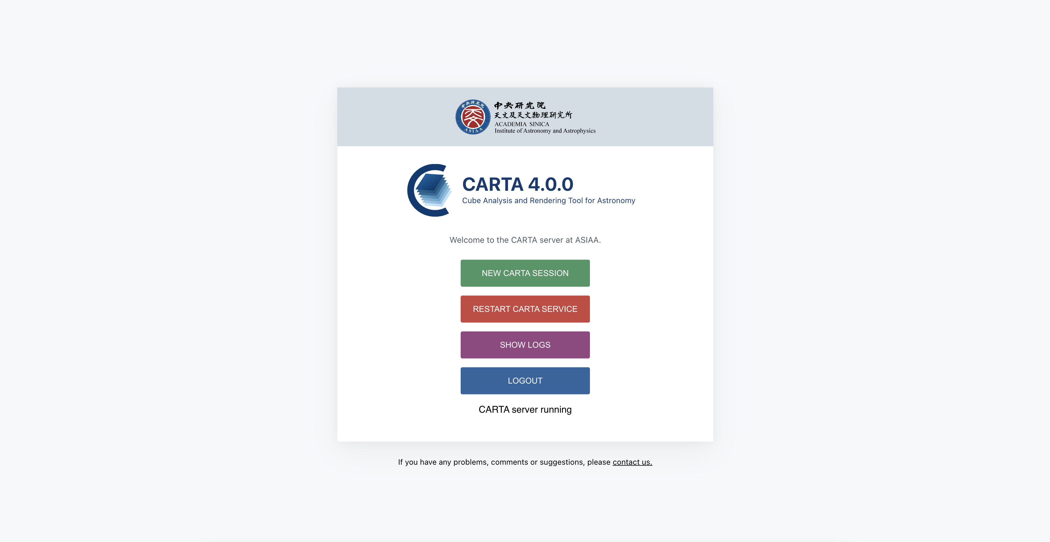
If you are using the Site Deployment Mode (SDM) of CARTA and encountering the case that the backend is not accessible, you can go to the dashboard to restart a CARTA service. The dashboard can be also visited also via the menu “File” -> “Server” -> “Dashboard” in normal state. With the dashboard, you can

• Start a new CARTA session (using the same backend)

• Restart a CARTA service (a.k.a., backend)

• Show backend log

• Logout

Note that the dashboard may look differently per site deployment.

File Browser

The File Browser, accessible via the menu “File” -> “Open Image” or the menu “File” -> “Append Image”, provides a list of images and their information supported by CARTA. The supported image formats are:

• CASA format

• HDF5 format (IDIA schema)

• FITS format

• MIRIAD format

Only images that match these formats will be shown in the file list by default. If you usually work with directories containing lots of files, you may switch to a different file list generation mode via “File” -> “Preferences” -> “Global” -> “File List”. The performance of the file list generation can be improved by just using the file extension as the parser or by simply listing all files without parsing the image type.

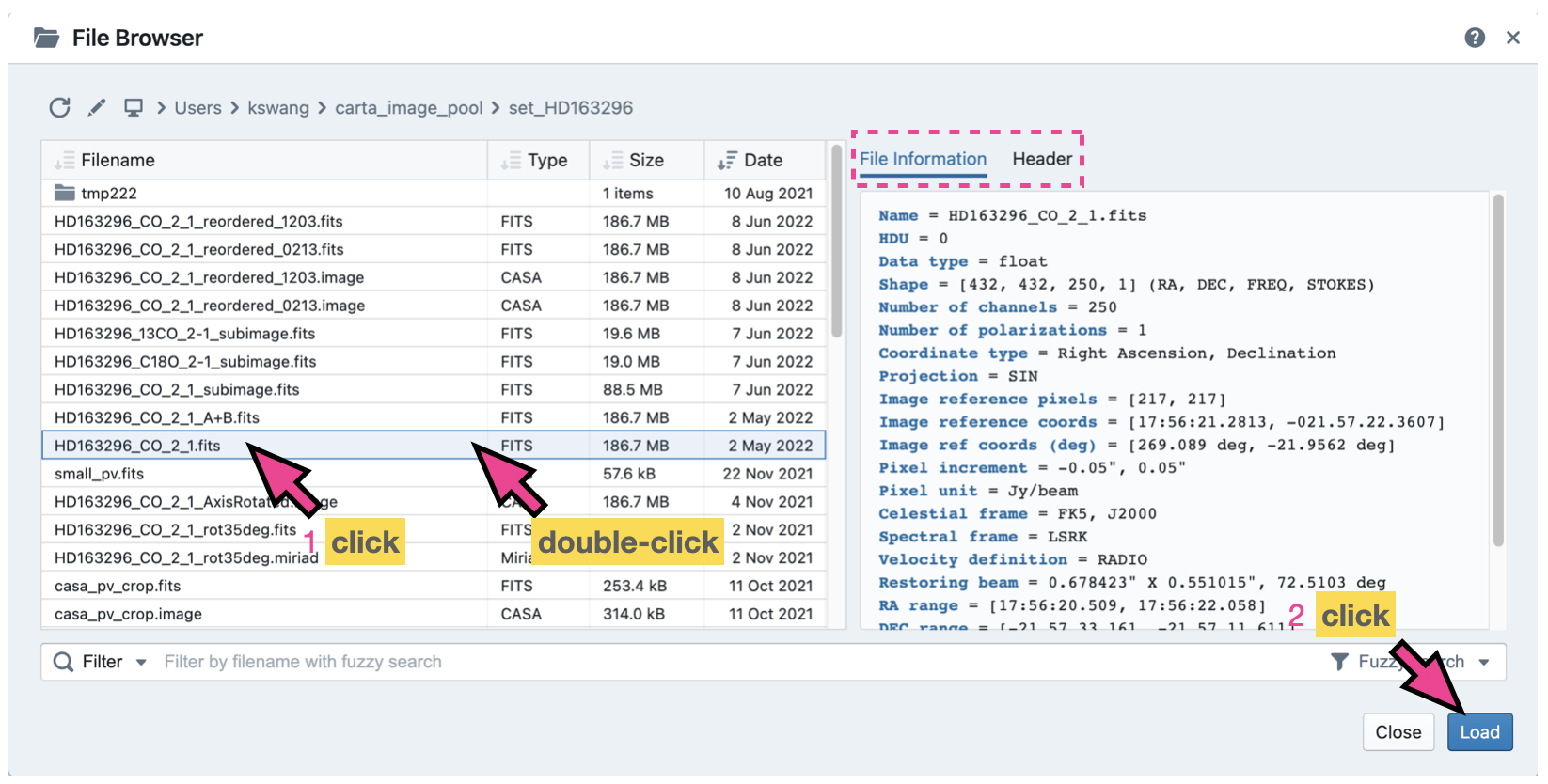
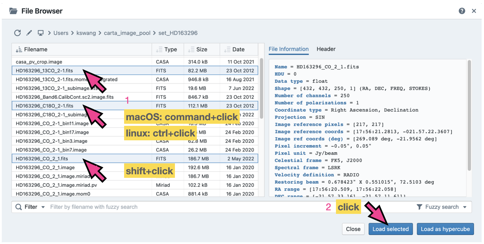
When an image is selected, a summary of image properties is provided on the right-hand side of the dialog. The full image header is available in the second tab. To view an image, click the “Load” button at the bottom-right corner. You can also double-click an image to load it directly. To view a new image and close all the loaded images, use the “File” -> “Open Image” -> “Load” button. To view a new image without closing all the loaded images, use the “File” -> “Append Image” -> “Append” button.

If multiple images are required to perform joint visualization and analysis (e.g., CO 2-1, 13CO 2-1, and C18O 2-1), you can select multiple files in the file list with “shift+click”/”command+click” (macOS) or “shift+click”/”ctrl+click” (Linux) and load or append them all at once.

You can search for files and sub-directories using the filter field located at the bottom of the File Browser. Three different methods are supported:

• Fuzzy search: free typing

• Unix pattern: e.g., *.fits

• Regular expression: e.g., colou?r

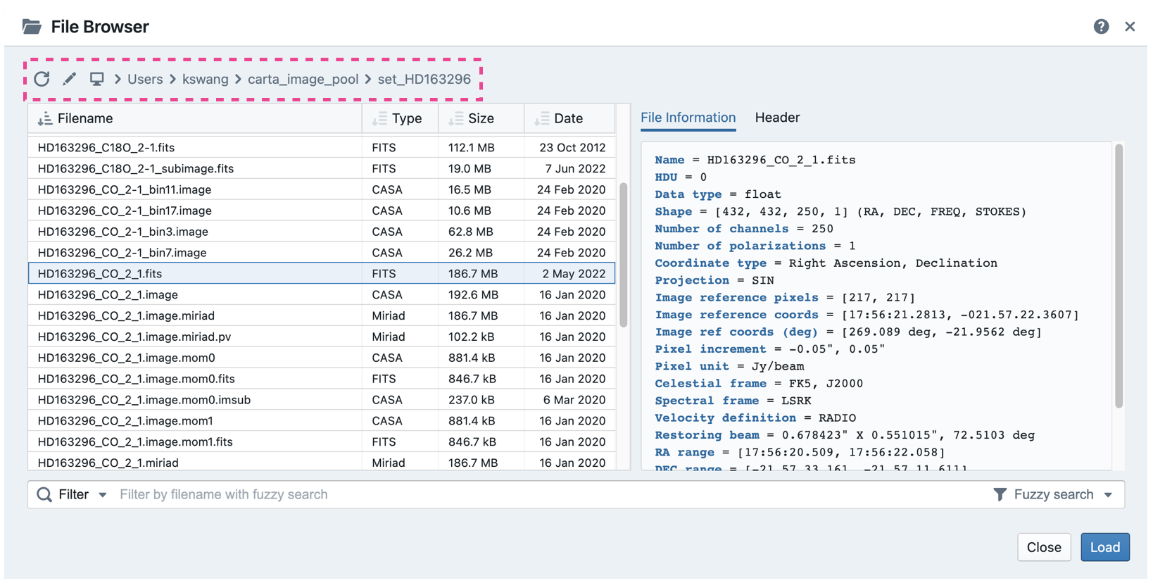
The File Browser remembers the last path where an image was opened within one CARTA session, and the path is displayed (as breadcrumbs) at the top of the File Browser. Therefore, when the File Browser is re-opened to load other images, a file list will be displayed at the path where the previous image was loaded. CARTA can also remember the last path for a new CARTA session via “File” -> “Preferences” -> “Global” -> “Save last used directory”.

You can use the breadcrumbs to navigate to one of the parent directories or click the home button to directly navigate to the base (i.e., initial) directory. Alternatively, you can use the pencil button and enter a path directly to switch directories. You can click the reload button to get an updated file list from the server side.

Note

For the CARTA deployed in the “Site Deployment Mode”, the server administrator can limit the global directory access through the --top_level_folder flag when a CARTA backend service is initialized.

exec carta_backend /scratch/images/Orion --top_level_folder /scratch/images

In the above example, you will see a list of images at the directory “/scratch/images/Orion” when you access the File Browser Dialog for the first time in a new session. You can navigate to any other folders inside “/scratch/images/Orion”. You will navigate to the directory “/scratch/images/Orion” directly by clicking the home button. You can also navigate one level up to “/scratch/images”, but not beyond that (neither “/scratch” nor “/”) as limited by the --top_level_folder flag.

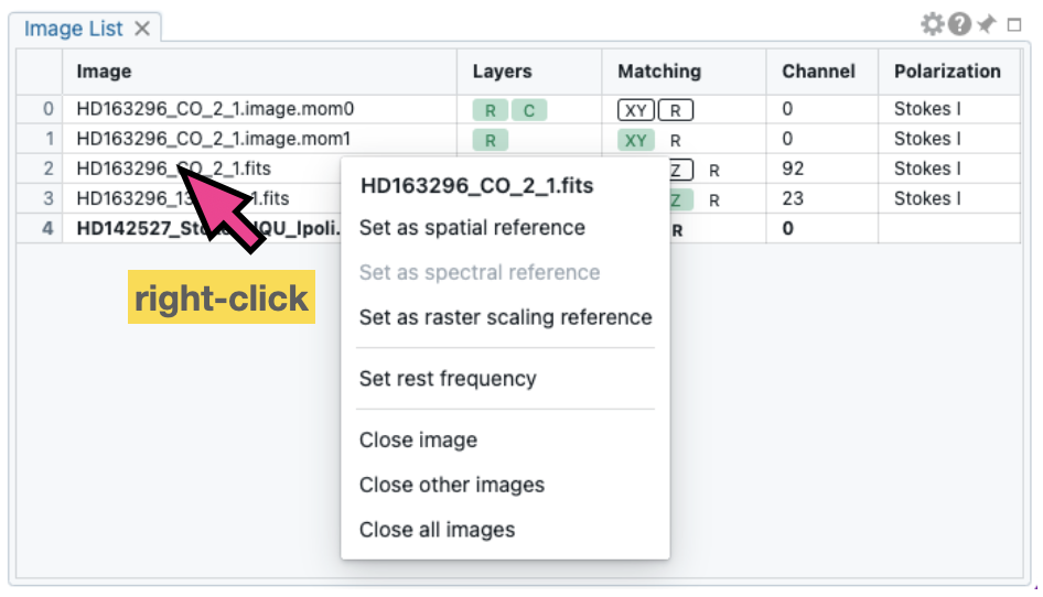
An image can be closed via “File” -> “Close Image”. The active image (the image in the single-panel view or the image highlighted with a red box in the multi-panel view) will be closed. Alternatively, you can close an image via the context menu (right-click) in the Image List Widget. Note that if the image being closed is a WCS reference image, any other matched images to this reference image will be unmatched. Therefore, they will be just like individual images.

Tip

An image may be opened directly using a modified URL. For example, if you want to open an image file “/home/acdc/CARTA/Images/jet.fits”, you can append

&folder=/home/acdc/CARTA/Images&file=jet.fits

or

&file=/home/acdc/CARTA/Images/jet.fits

to the end of the URL (e.g., http://192.168.0.128:3002/?token=E1A26527-8226-4FD5-8369-2FCD00BACEE0). In this example the full URL is

http://192.168.0.128:3002/?token=E1A26527-8226-4FD5-8369-2FCD00BACEE0&folder=/home/acdc/CARTA/Images&file=jet.fits

or

http://192.168.0.128:3002/?token=E1A26527-8226-4FD5-8369-2FCD00BACEE0&file=/home/acdc/CARTA/Images/jet.fits

Please note that it is necessary to supply a full path. Tilde (~), as your home directory, is not allowed.

Note

CARTA image loading performance

The per-channel rendering approach helps to improve the performance of loading an image. Traditionally, when an image is loaded, the minimum and maximum of the entire image (cube) are computed first before image rendering. This becomes a severe performance issue if the image (cube) size is huge (more than a few tens to hundreds of GB). In addition, applying the global minimum and maximum to render a raster image usually (if not often) results in a poorly rendered image if the dynamic range is high. Then, you will need to re-render the image repeatedly with refined boundary values. Re-rendering such a large image repeatedly with CPUs further deduces user experiences.

CARTA improves the image viewing experience by adopting GPU-accelerated rendering techniques in the web browser environment. In addition, CARTA only renders an image with sufficient image resolution (image tiles with a proper down-sampling factor) for your screen. This combination results in a scalable and high-performance remote Image Viewer. The total file size is no longer a bottleneck. The determinative factors are 1) image size in x and y dimensions, 2) internet bandwidth, and 3) storage I/O performance, instead. For a laptop with 8 GB of RAM, the largest image it can load without memory swapping is about 40000 pixels by 40000 pixels (assuming most of the RAM is free before loading the image).

The approximated RAM usage for loading images with various spatial sizes is summarized below.

Image size (x, y) [pixel]	RAM usage
512	1 MB
1024	4 MB
2048	16 MB
4096	64 MB
8192	256 MB
16384	1 GB
32768	4 GB
65536	16 GB

HDF5 (IDIA schema) image support

Besides the CASA image format, the FITS format, and the MIRIAD format, CARTA also supports images in the HDF5 format under the IDIA schema. The IDIA schema is designed to ensure efficient image visualization is retained even with huge image cubes (hundreds of GB to a few TB). The HDF5 image file contains extra data to skip or speed up expensive computations, such as per-cube histogram, spectral profile, etc. Below is a summary of the content included in an HDF5 image:

• XYZW dataset (spatial-spatial-spectral-Stokes): similar to the FITS format

• ZYXW dataset: rotated dataset

• Per-channel statistics: basic statistics of the XY plane

• Per-cube statistics: basic statistics of the XYZ cube

• Per-channel histogram: histogram of the pixel values of the XY plane

• Per-cube histogram: histogram of the XYZ cube

• Per-channel mip map: downsampled image tiles

The CARTA development team provides a FITS-to-HDF5 converter for you to convert a FITS image to the HDF5 (IDIA schema) format. You can refer to Installation of fits2idia (converting FITS to HDF5-IDIA) on how to install fits2idia program on your platform.

The fits2idia usage is the following:

IDIA FITS to HDF5 converter version 0.1.15 using IDIA schema version 0.3
Usage: fits2idia [-o output_filename] [-s] [-p] [-m] input_filename

Options:
-o   Output filename
-s   Use slower but less memory-intensive method (enable if memory allocation fails)
-p   Print progress output (by default the program is silent)
-m   Report predicted memory usage and exit without performing the conversion
-q   Suppress all non-error output. Deprecated; this is now the default.

Note

Currently the per-plane beam table is not supported in the HDF5 (IDIA schema) format.

Forming a Stokes hypercube

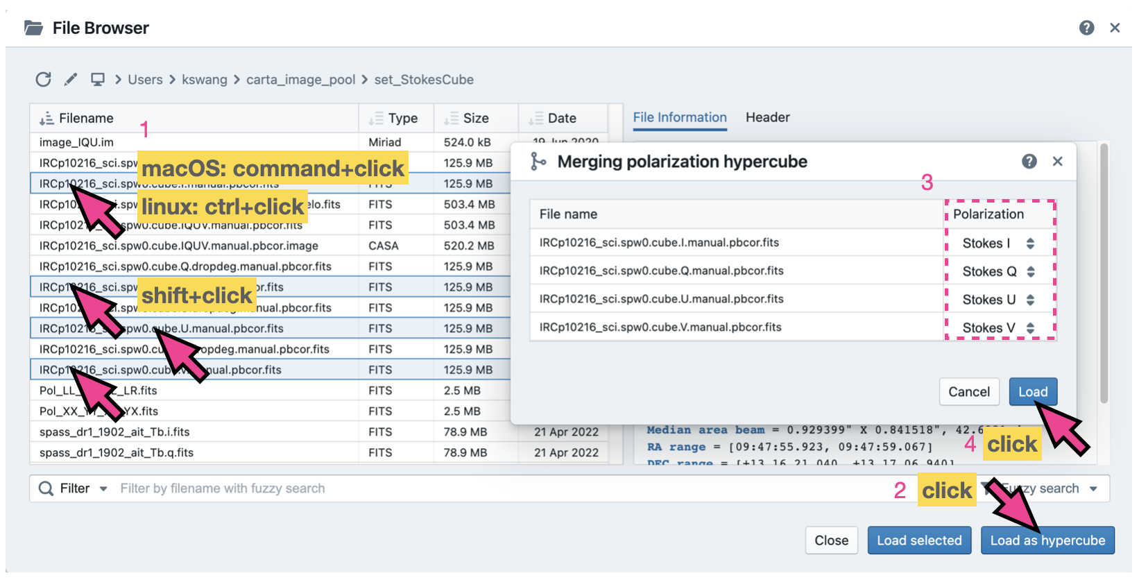
Suppose a set of individual Stokes images needs to be loaded into CARTA for data inspection with the Stokes Analysis Widget. In that case, you can multi-select individual Stokes images (e.g., image_I.fits, image_Q.fits, image_U.fits, and image_V.fits) in the file list with “shift+click”/”command+click” (macOS), or “shift+click”/”ctrl+click” (Linux), and load them with the “Load as hypercube”. A dialog will show up for you to confirm the identification (based on image headers or file names) of the Stokes parameters of the selected images. After clicking the “Load” button, the backend will form a hypercube from the selected images. Effectively, only one (virtual) image with multiple Stokes parameters is loaded in CARTA.

If you need to save a Stokes hypercube as an image file, go to the “File” menu and select “Save Image”.

Loading images with the Lattice Expression Language (LEL)

CARTA supports loading images via the Lattice Expression Language (LEL) interface. To enable this feature, click the “Filter” dropdown menu in the File Browser and switch to the “Image arithmetic” mode. Please refer to the Lattice Expression Language for detailed usages.

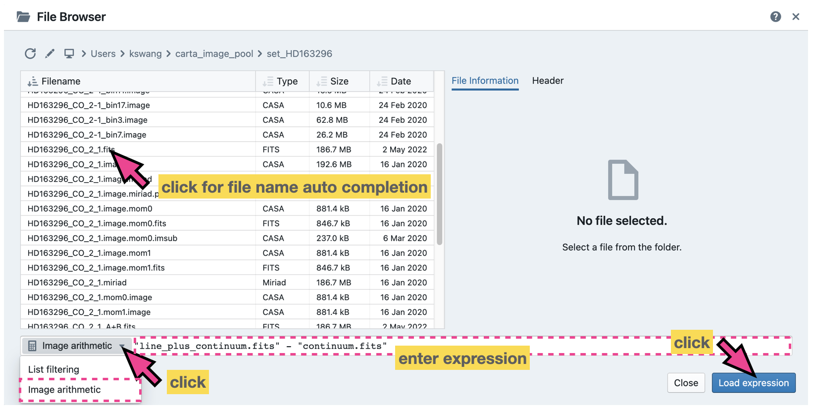
With the LEL interface, you can apply arithmetic on images and load the result as an image in CARTA. For example, with the expression

"line_plus_continuum.fits" - "continuum.fits"

a “line only” image will be computed and loaded in CARTA.

When the LEL interface is enabled, you can either manually enter the expression in the expression field or use a mouse click to auto-complete an image file name to speed up the process.

If you need to save the image computed via the LEL interface, go to the “File” menu and select “Save Image”.

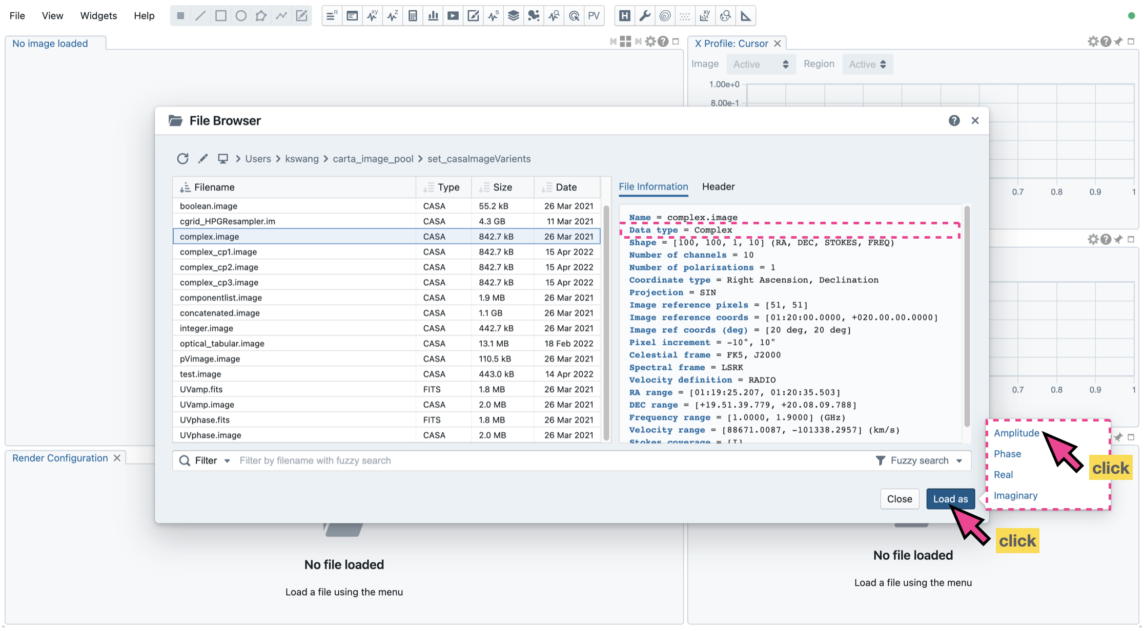
Loading a complex-valued image

A complex-valued CASA image is supported in CARTA. When a CASA image is detected as complex-valued, the “Load as” button includes the following components:

• Amplitude

• Phase

• Real

• Imaginary

as loading options. You can select a desired component to load or append.

If you want to save a component (e.g., Amplitude) as a new image file with the float data type, go to the “File” menu and select “Save Image”.

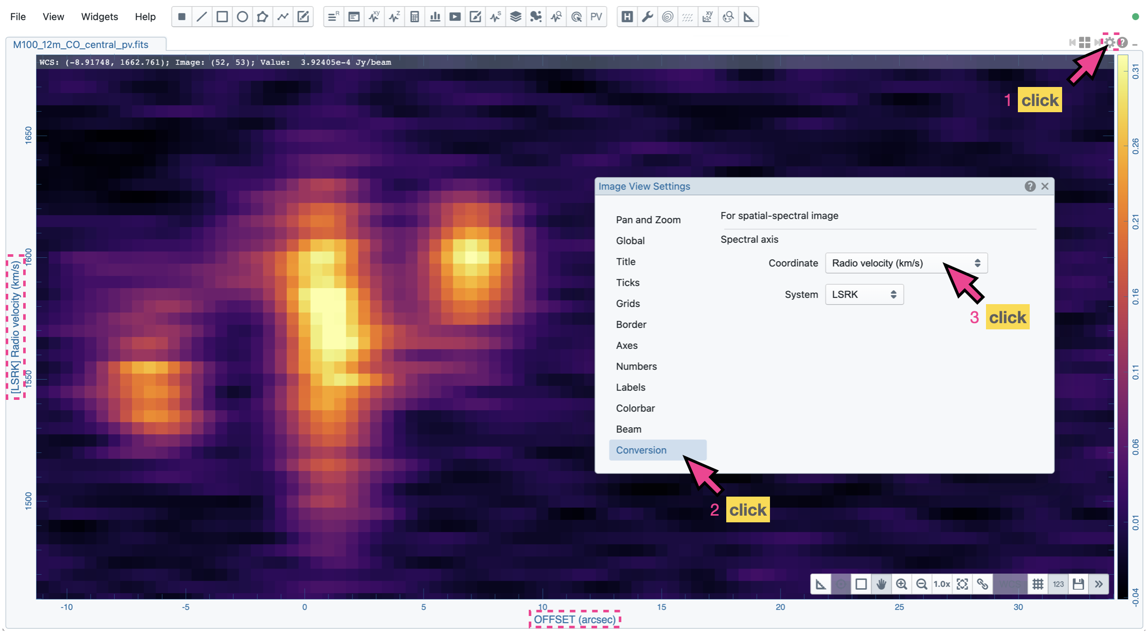
Loading a Position-Velocity (PV) image

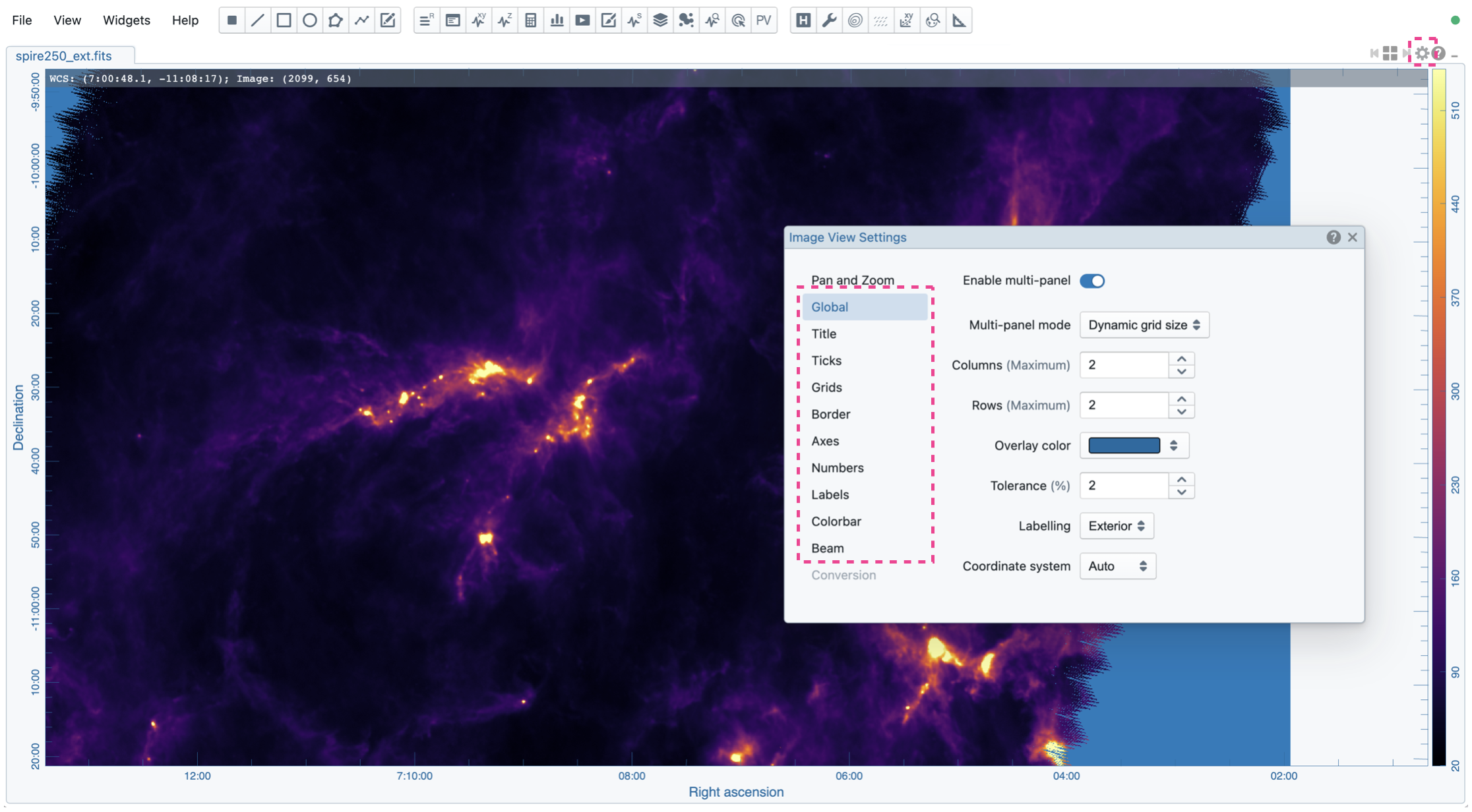
You can load a position-velocity (PV) image in CARTA. When the image header has sufficient information for the spectral conversion of the “V” axis (e.g., velocity <-> frequency), you can apply the conversion via the “Conversion” tab of the Image Viewer Settings Dialog (the “cog” button at the top-right corner of the Image Viewer Widget).

Loading a swapped-axes image cube

CARTA supports a swapped-axes image cube. When such a cube is selected in the file list, the file information panel will show the labels of the axes in order. The first two axes will be used for rendering the XY plane in the Image Viewer. The Stokes axis (if there is any) will still be interpreted as a polarization axis. The third axis (excluding the Stokes axis, if there is any) will be interpreted as the Z axis for animation playback. In the following example, CARTA will render a FREQ-RA image in the Image Viewer. With the Animator Widget, you can trigger animation playback of the DEC axis (or the polarization axis, if there is any).

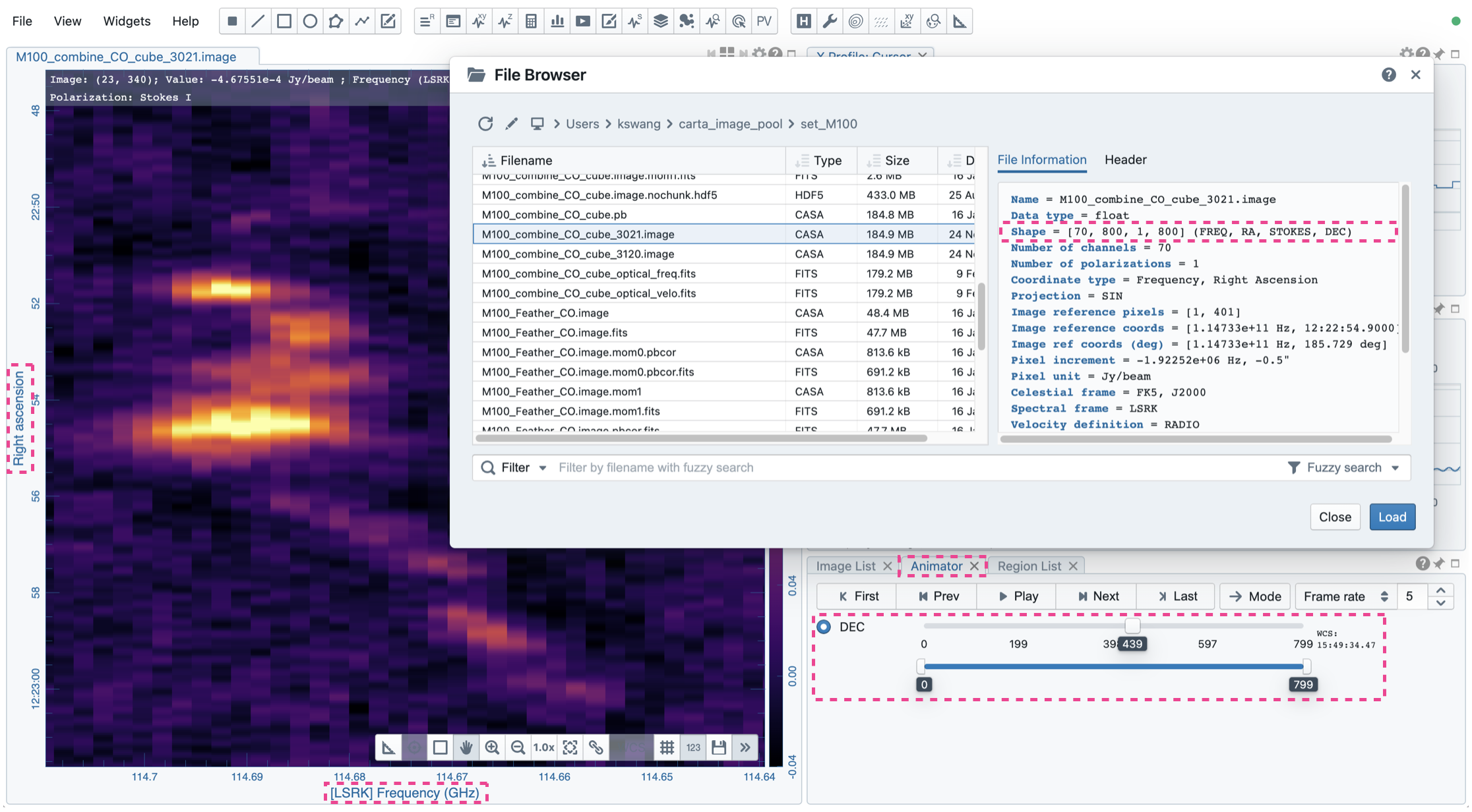
Warning

In v4.1.0, CARTA supports swapped-axes image cubes for image visualization only. Region analytics tools are not supported.

Image viewer

Warning

If you run a VNC session from a headless server, CARTA may fail to render images correctly (they may appear as a block with a uniform color or as an empty plot). It is because CARTA renders images using WebGL2, which uses GPU to accelerate the rendering process. Most headless servers have neither discrete nor integrated GPUs. In such cases, it is highly recommended to use your local web browser to access the backend, as it is much more efficient than VNC. Please refer to the section How to run CARTA?.

CARTA can render images in different ways, such as:

1. a single raster image

2. a single raster image plus its contours

3. a single raster image plus a set of contour images with matched world coordinates from other image files

4. a set of contour images without a background raster image

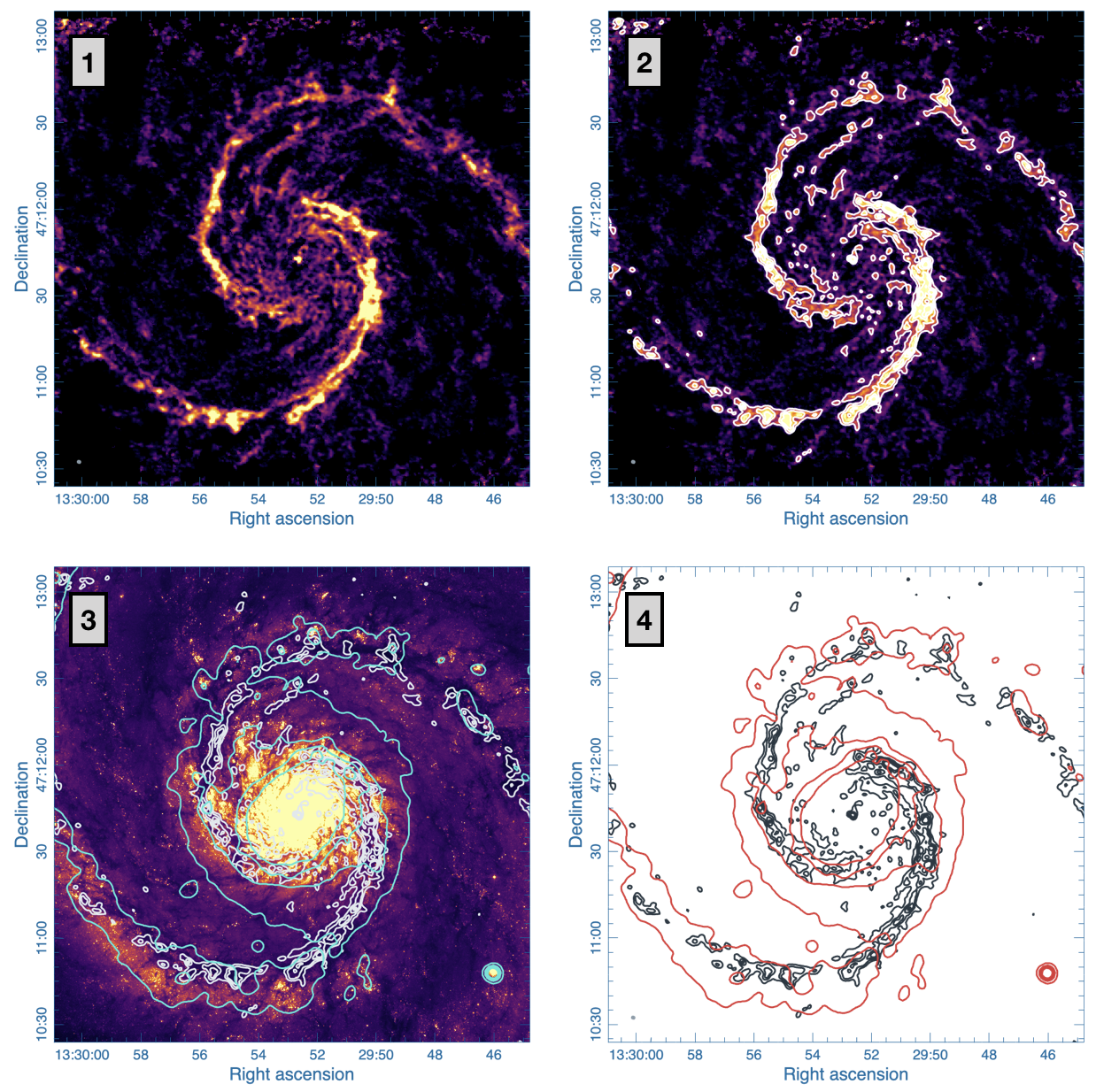
By default, CARTA displays images as raster images when loaded, like the first example in the figure above. You then can generate contour images (see Contour rendering) and enable WCS matching between different images (see Matching images spatially and spectrally), such as the other three examples above.

In addition, a vector overlay from a vector field (e.g., a linear polarization field or a magnetic field, etc.) or a scalar field (e.g., a temperature field or a column density field, etc.) can be added to the image view (see Vector field rendering).

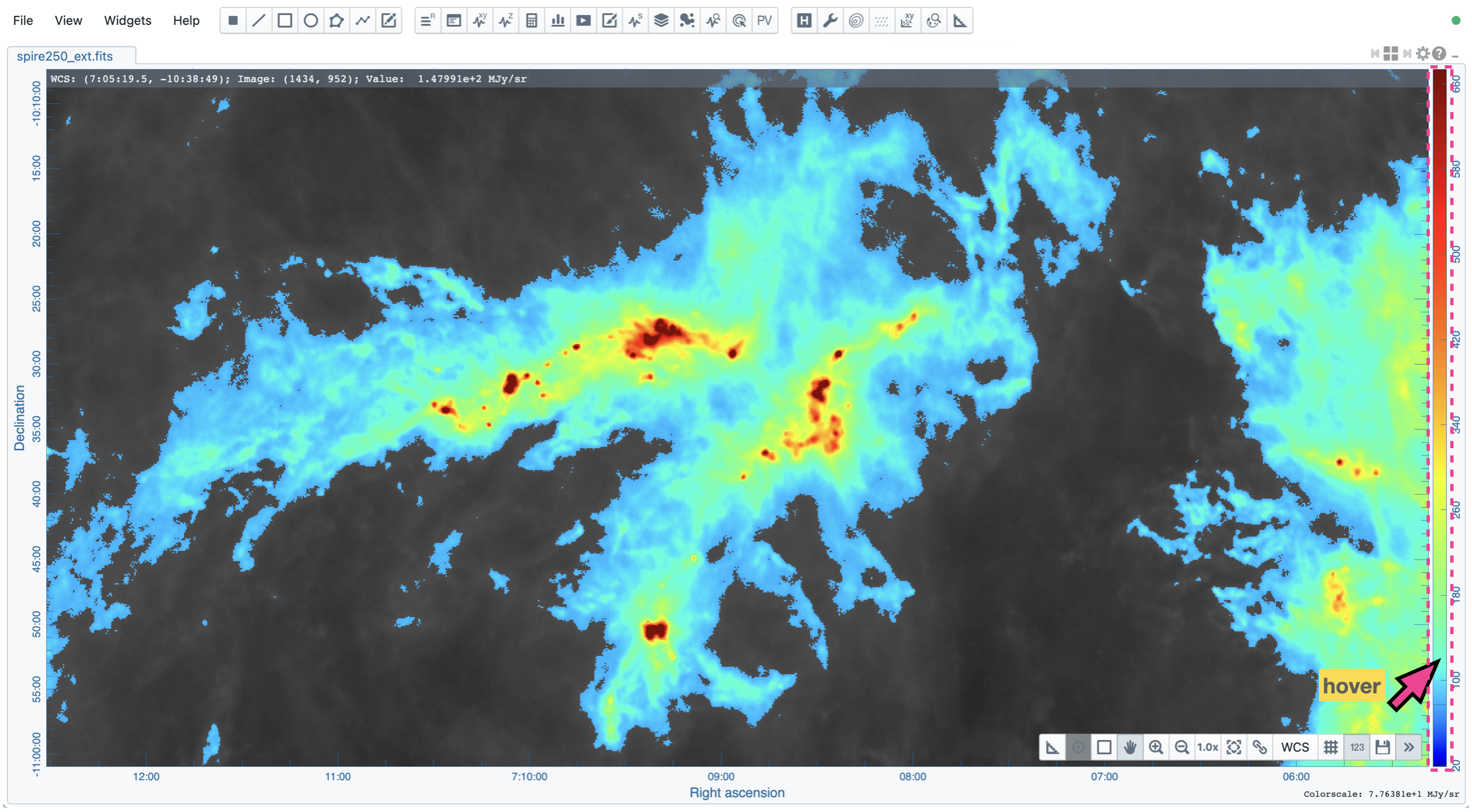
By default, a colorbar is displayed along with the raster image on the right-hand side. You can configure its properties in the settings dialog (the “cog” button at the top-right corner) of the Image Viewer Widget. In “File” -> “Preferences” -> “WCS and Image Overlay”, you can set colorbar properties persistent for new images, such as the orientation of the colorbar, for example. When you use the mouse to hover over the colorbar, a color-scale value is displayed at the bottom of the colorbar, and a real-time color clip of the color-scale value is applied to the Image Viewer to assist you in investigating features in the image. The pixels less than the color-scale are rendered in grayscale temporarily. This interactive feature can be disabled in “File” -> “Preferences” -> “WCS and Image Overlay”.

Note

Tiled rendering techniques

CARTA utilizes an efficient approach, “tiled rendering”, to display a raster image. In the Image Viewer, you see an ensemble of image tiles (default 256 pixels by 256 pixels) processed in parallel.

As shown in the figure below, if we have an image with 2048 pixels by 2048 pixels, tiles will be constructed in four layers with different downsample factors. The zeroth layer contains only one tile with a size of 256 pixels by 256 pixels. A downsample factor of 8 is applied to the original image to create this tile. The first layer contains four tiles, each with a size of 256 pixels by 256 pixels. The downsample factor of 4 is applied to the original image to create these four tiles. This process continues until no downsampling is required. In this case, the tiles of the third layer are not downsampled.

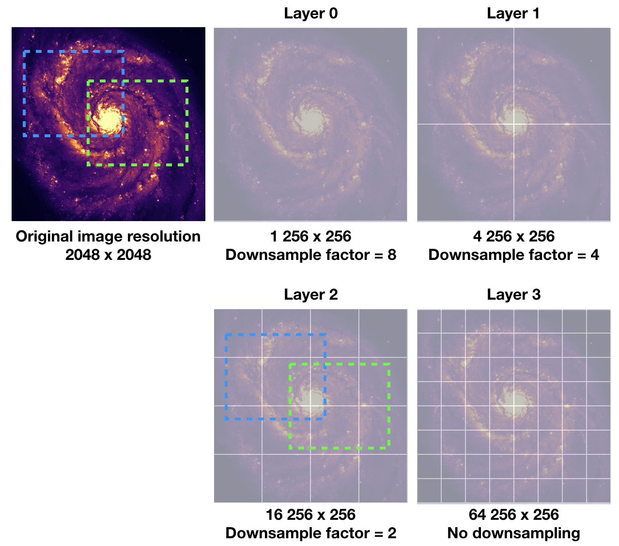
When you change the field of view or the size of the Image Viewer, tile data of the right layer matching your screen resolution will be used. For example, if you are interested in the field of the blue box and the Image Viewer has a screen size of 512 pixels by 384 pixels, tiles of the 2nd layer will be used for rendering. In this case, nine tiles will be used. If you pan a little bit around the blue box, no new tile data are required. However, if you pan the view to the green box with the same viewer size, two additional tiles from the second layer are required, and four tiles will be re-used for rendering. With this tiled rendering approach, tiles will be re-used at different zoom levels and with different fields of view to minimize the amount of data transfer while keeping the image sharp on the screen. Effectively, you will see that the image becomes sharper and sharper at higher and higher zoom levels.

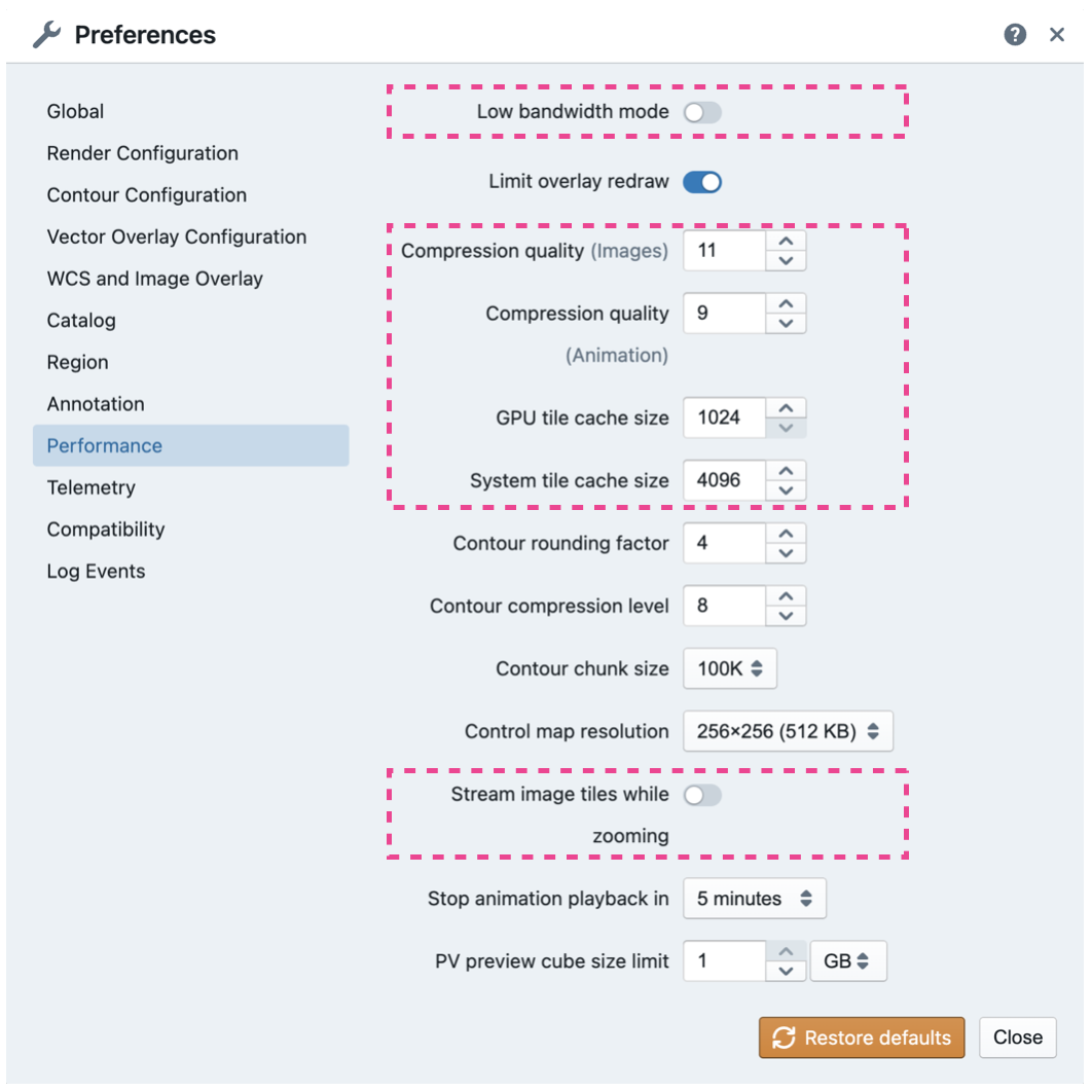
The performance of the tiled rendering can be customized with the Preferences Dialog, “File” -> “Preferences” -> “Performance”. The default values are chosen to ensure that raster images are displayed efficiently with sufficient accuracy. Advanced users may refine the setup if necessary. For example, when accessing a remote backend under poor internet conditions, the compression quality might be slightly lowered to make the tile data smaller. Note that a lower compression quality might introduce noticeable artifacts on the raster image. Please adjust with caution.

Alternatively, you may enable the low bandwidth mode, which will reduce required image resolutions by a factor of two (so that the image will look slightly blurry) and cursor responsiveness from 200 ms to 400 ms (HDF5 images: from 100 ms to 400 ms). Under good internet conditions, you may enable streaming image tiles while zooming to see progressive updates of image resolutions at different zoom levels.

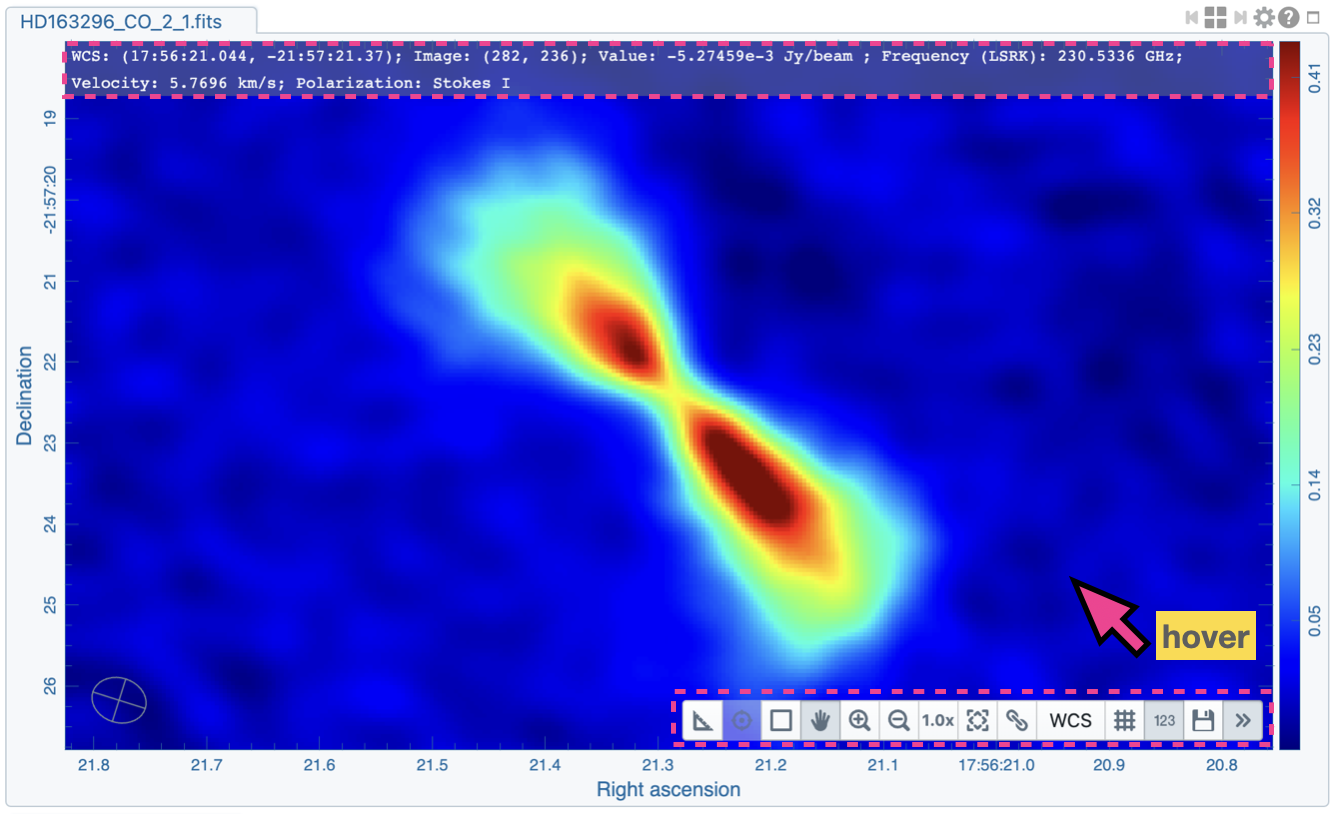
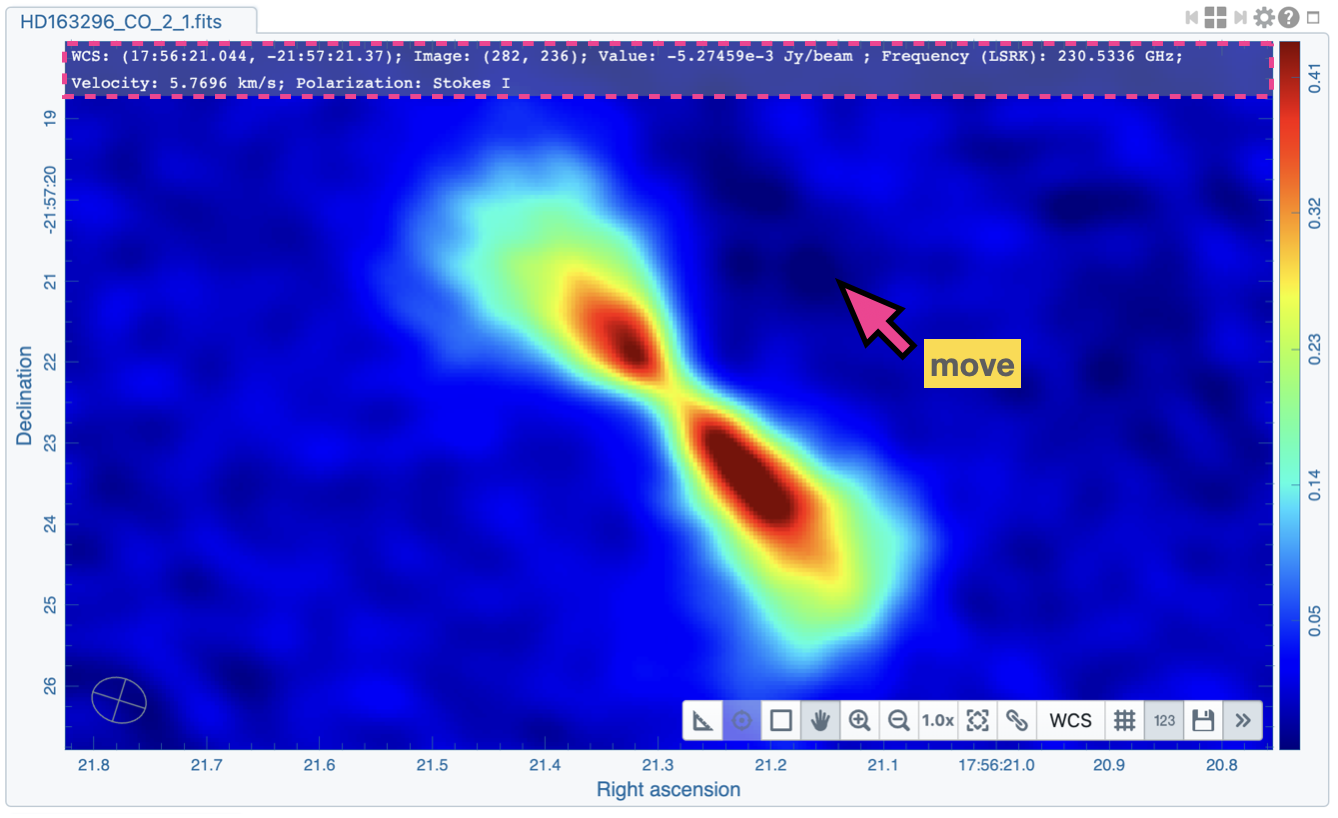
In addition to displaying images, the Image Viewer displays cursor information at the top and provides a set of tool buttons in the bottom-right corner when you use the mouse to hover over the image.

Tip

A cursor info bar is displayed at the top of the active image plot by default in the Image Viewer. When it is the single-panel view mode, the image in the current view is the active image. When it is the multi-panel view mode, the active image is highlighted with a red box. With the “File” -> “Preferences” -> “WCS and image overlay” -> “Cursor Info Visible” dropdown menu, you can switch to a different mode. Available modes are

• Always: Always show the cursor info bar per image

• Active image only: Only show the cursor info bar on the active image (default)

• Hide when tiled: Do not show the cursor info bar when it is in the multi-panel view mode.

• Never: Do not show the cursor info bar regardless of whether it is the single-panel view mode or the multi-panel view mode.

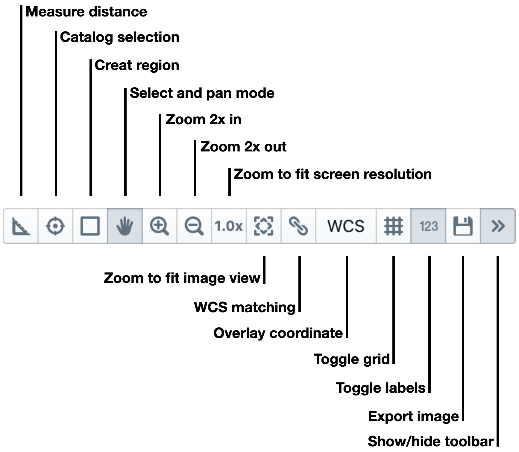
The tool buttons allow you to

• measure an angular distance

• select a source from the catalog overlay (if applicable)

• create a region of interest or an annotation object

• perform zoom actions

• enter pan mode

• trigger matching images in world coordinates and/or in the spectral domain

• change reference coordinate grid lines and labels

• export image as a PNG file

• hide/show the toolbar

The widget geometry determines the aspect ratio of the image view. When the Image Viewer Widget is resized, a tooltip with a ratio in screen pixels will be displayed (c.f., Resizing a widget ).

When the cursor is movning on the Image Viewer, the pixel information at the cursor position is shown at the top side of the image. The information includes:

• World coordinate of the current coordinate system.

• Image coordinate in pixel (0-based).

• Pixel value.

• Frequency, velocity, reference frame (if applicable), and polarization parameter (if applicable).

When the coordinate system changes (e.g., ICRS to GALACTIC), the displayed world coordinate will be changed accordingly. By default, they are displayed in decimal degrees for GALACTIC and ECLIPTIC systems, while for FK5, FK4, and ICRS systems, they are displayed in sexagesimal format. The precision of both formats is determined dynamically based on the image header and the image zoom level.

The reference image coordinate (0, 0) is located at the center of the bottom-left pixel of the image. Whether the displayed image is downsampled, the image coordinate always refers to the full-resolution image.

When the cursor is moving, a pixel value of the full-resolution image is displayed. If the image header provides sufficient information in the frequency/velocity domain, a frequency and a velocity with the reference frame of the current channel will be shown. A polarization parameter (e.g., Stokes I) will also be displayed if the polarization information is available in the image header.

To stop/resume cursor update, press the “F” key. When the cursor stops updating, the cursor information bar, cursor spatial profile, and cursor spectral profile will stop updating, too.

Single-panel view and multi-panel view

The Image Viewer provides two modes for viewing images: single-panel and multi-panel views. By default, a dynamic multi-panel view mode is enabled. You can use the “viewer mode” button at the Image Viewer Widget’s top-right corner to switch between the two modes. The view mode is persistent in a new CARTA session (i.e., it is an implicit preference). Additional view mode configuration options are available in the settings dialog of the Image Viewer Widget. You can have a dynamic multi-panel view layout (with a configurable maximum n rows by m columns) based on the number of loaded images or have a fixed layout regardless of how many images are loaded. You can use the “next page” and “previous page” buttons at the top-right corner of the Image Viewer to view images if the current grid layout cannot show all loaded images at once.

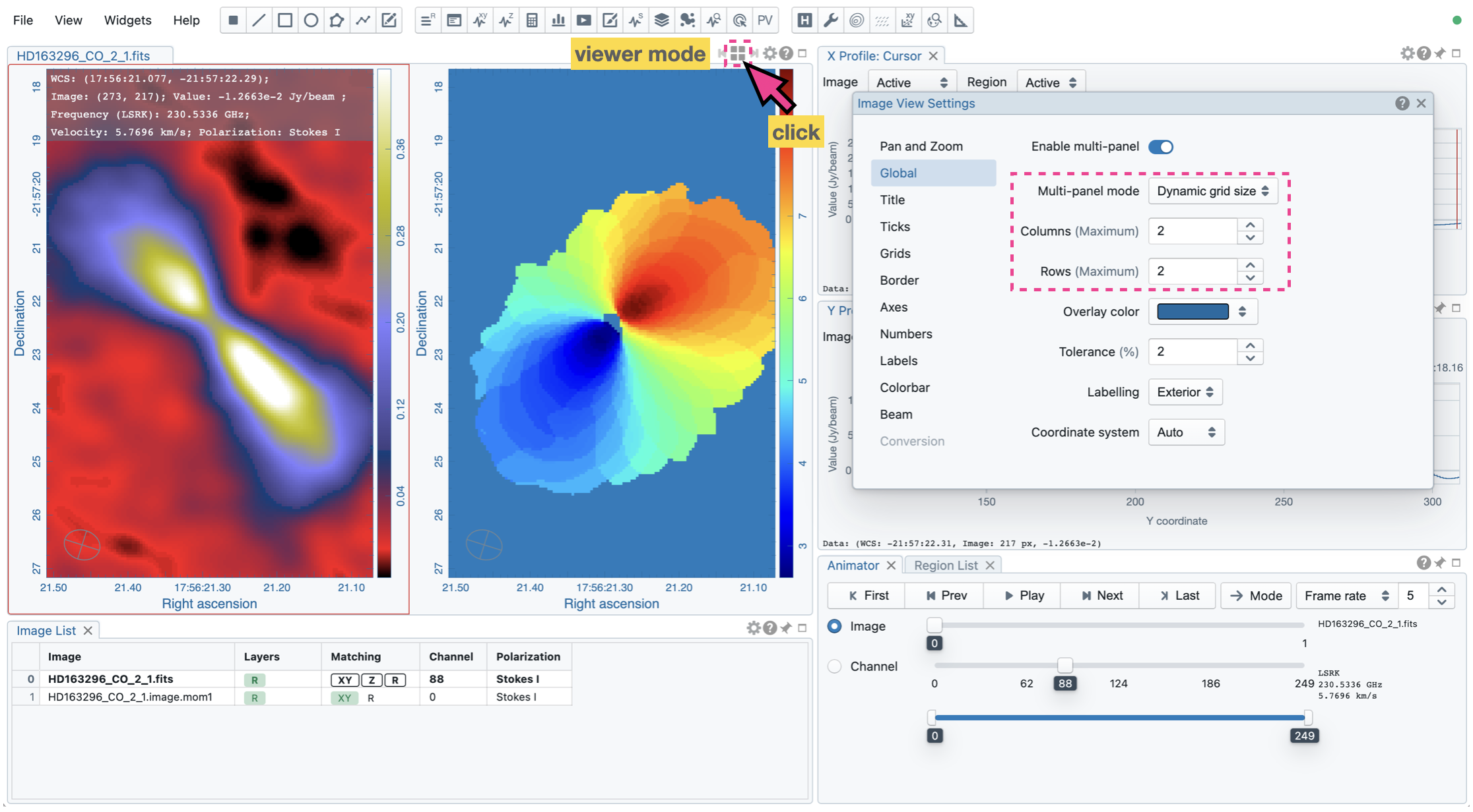
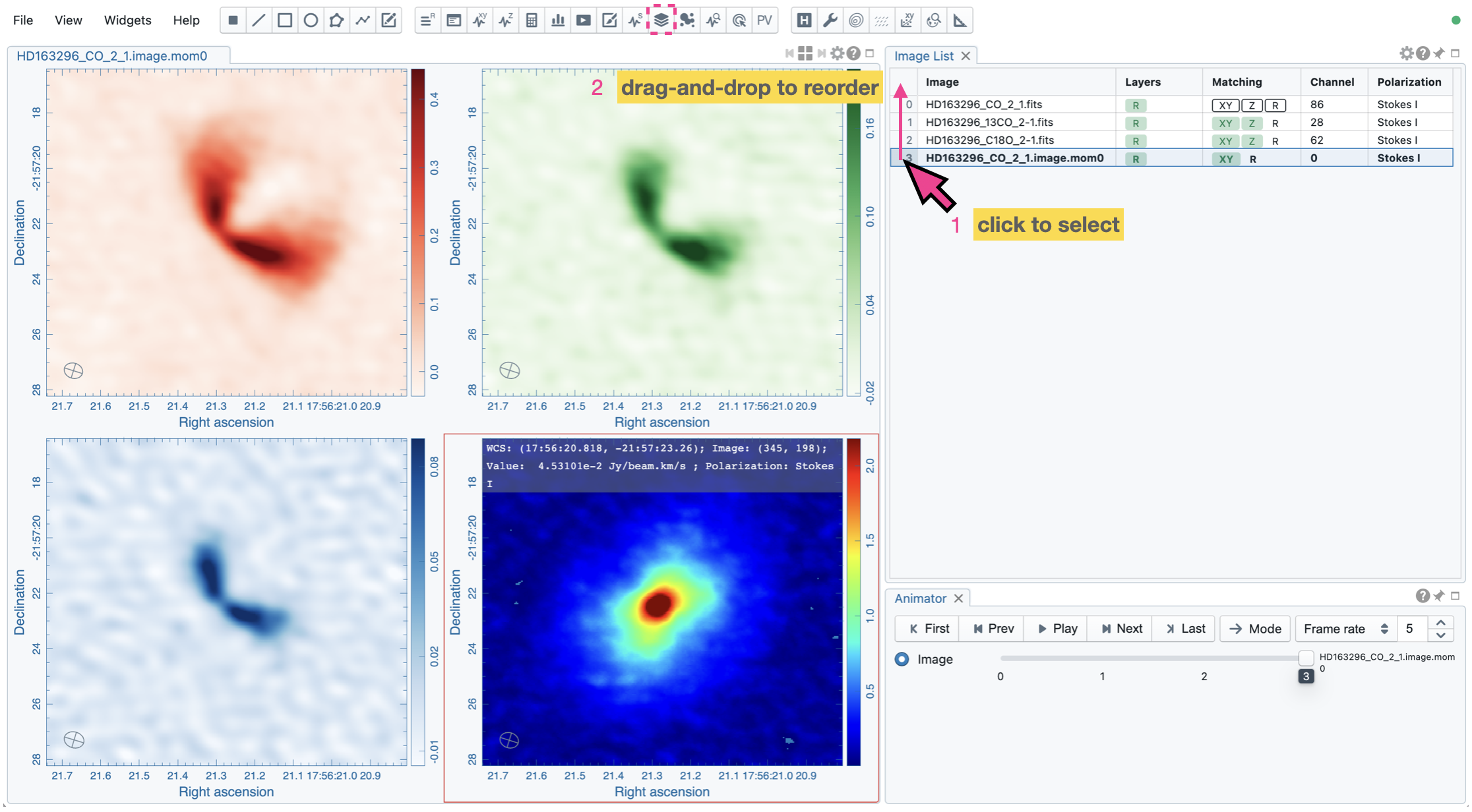
When the view mode is single-panel, the image in the view is the “active” image. The “active” image is highlighted with a red box when the view mode is multi-panel. In the above example, the image on the left-hand side is the “active” image. In the Image List Widget (the widget at the bottom-left corner in the above example), the “active” image is highlighted in boldface. There is always an “active” image, except when no image is loaded in CARTA. You can use the Animator Widget or the Image List Widget to select a new “active” image.

In analytics widgets, such as the Statistics Widget or the Spectral Profiler Widget, the “Image” dropdown menu contains a list of loaded images, as well as an option as “Active” (default), which refers to the “active” image in the Image Viewer. This feature allows you to view the “active” image’s analytics efficiently without needing extra configurations in all analytics widgets. If you use the “Image” dropdown menu to select an image other than “Active”, the analytics widgets will stop updating if you set a new “active” image. For example, you can enable two Statistics Widgets and use the “Image” dropdown menu to configure the widgets to show the statistics from two images, respectively.

Tip

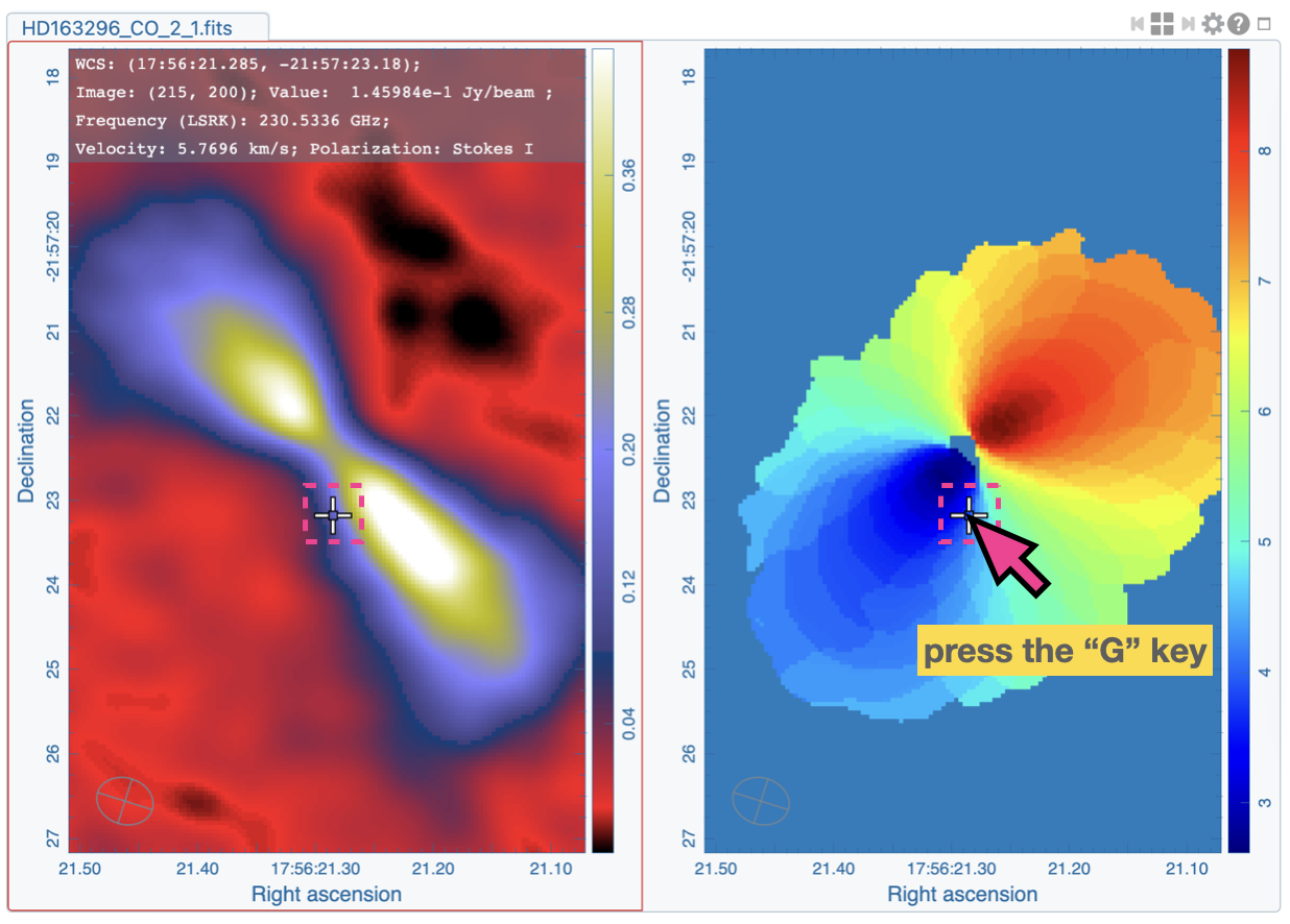
When comparing images side-by-side in the multi-panel mode, you can render mirrored cursor positions at different panels by clicking the “G” key.

Raster rendering

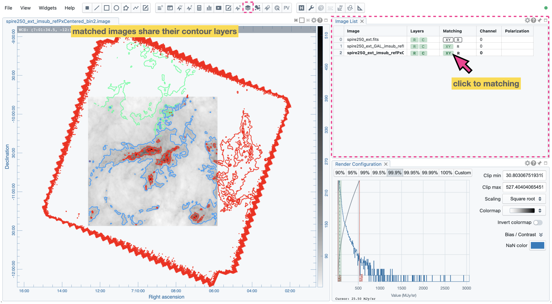
The Render Configuration Widget controls how a raster image is rendered in the Image Viewer. On the top is a row of buttons with different clip levels, plus a custom button. Below the clip buttons is a plot showing the per-channel histogram (with a logarithmic scale in y) with a bin count equal to the geometric mean of the image size (x and y). The two vertical red bars indicate the two clip values of a color map. The green dashed line marks the mean value, and the green box marks the range from mean minus one standard deviation to mean plus one standard deviation. The gray curve between the two red vertical bars shows the applied scaling function, including bias and contrast parameters. The mouse interaction with the histogram plot is summarized in the section Mouse interactions with charts.

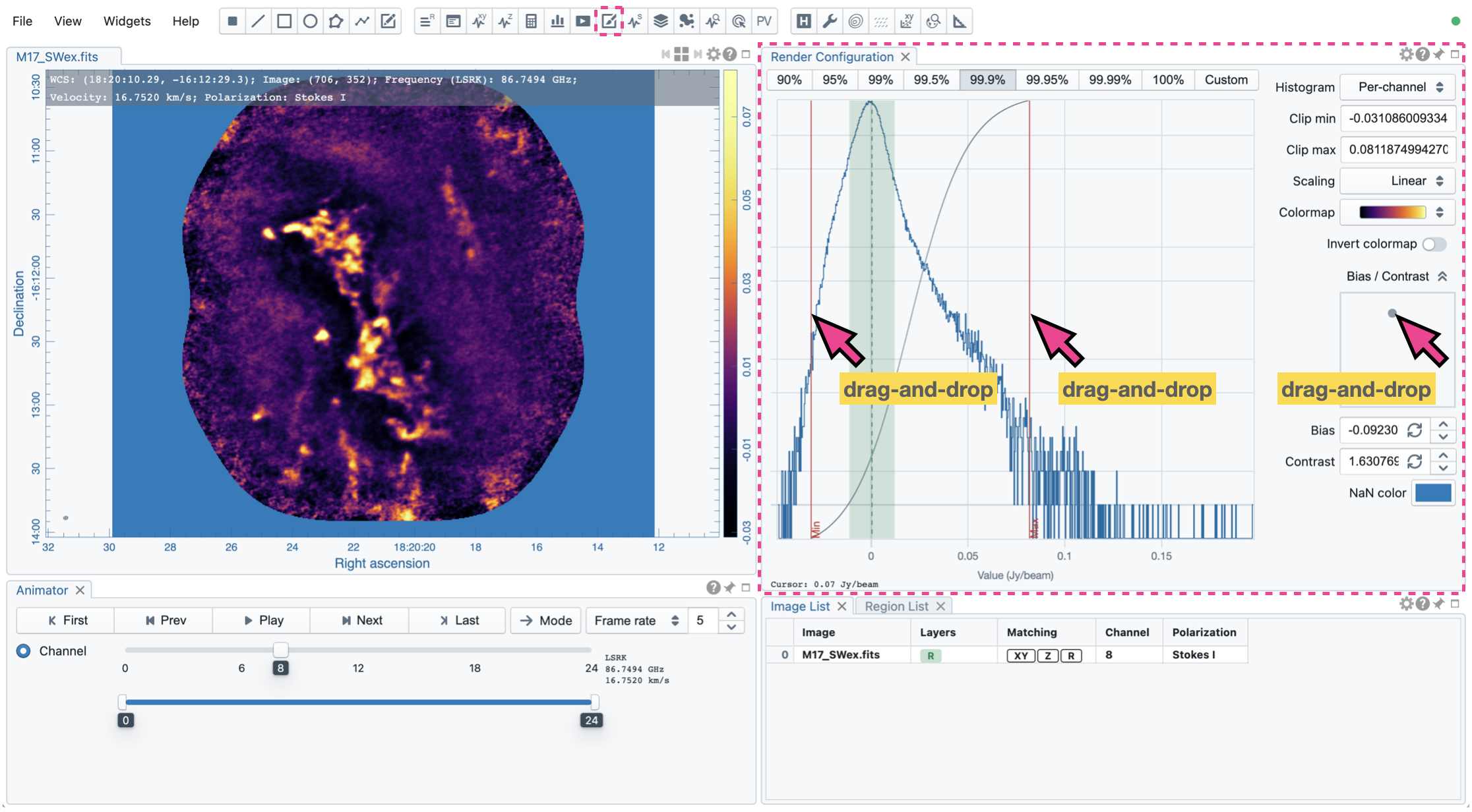
On the right-hand side of the Render Configuration Widget, there is a column of options, such as histogram type, scaling function, colormap, invert colormap, clip values, control parameter of a scaling function (if applicable), bias/contrast adjustment (i.e., a 2D box with x as bias and y as contrast), and NaN (not a number) color. Extra options to configure the histogram plot are placed in the settings dialog of the Render Configuration Widget, enabled by the “cog” button at the top-right corner of the Render Configuration Widget.

By default, CARTA calculates a per-channel histogram. When a per-cube histogram is requested, a warning message and a progress dialog will appear. Calculating a per-cube histogram can be time-consuming for large image cubes. You may cancel the request anytime by pressing the “cancel” button in the progress dialog. If the image is in the HDF5 format (IDIA schema), the pre-calculated per-cube histogram will be loaded and displayed instantly.

CARTA determines the boundary values of a colormap on a per-channel basis by default. A default “99.9%” clip level is applied to the per-channel histogram to look for the two clip values. Then, apply the values in a “linear” scale with zero bias and zero contrast to the default colormap “inferno” to render a raster image. This default procedure usually helps inspect an image in detail without suffering from improper image rendering.

However, color scales need to be fixed when comparing images channel by channel. You can drag the two vertical red bars or type in the values in the “Clip min” and “Clip max” input fields to do so. When this happens, the “custom” button is enabled automatically, and all channels will be rendered with the fixed boundary values. By clicking one of the clip buttons, CARTA switches back to the per-frame rendering mode if a per-channel histogram is requested. You may request the per-cube histogram to determine proper clip values.

CARTA provides a set of scaling functions, including:

• linear: \(y = x\)

• log: \(y = {\log}_{{\alpha}x+1}({\alpha}x+1)\)

• square root: \(y = {\sqrt{x}}\)

• squared: \(y = x^2\)

• gamma: \(y = x^{\gamma}\)

• power: \(y = ({\alpha}^x-1)/({{\alpha}-1})\)

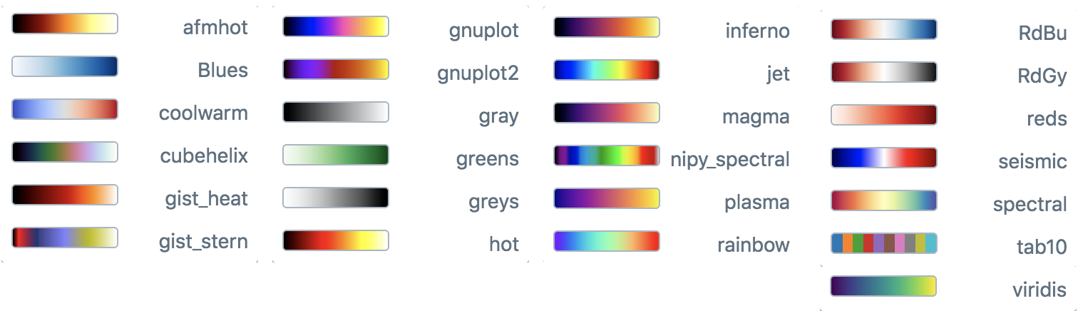
A set of color maps adopted from matplotlib is provided in CARTA.

The default scaling function, colormap, percentile rank (clip level), and color for NaN pixels can be customized via the menu “File” -> “Preferences” -> “Render Configuration”. When the “Smoothed bias/contrast” toggle is disabled, bias and contrast are applied so the resulting scaling function is piecewise smooth.

Note

Viewing a position-velocity image

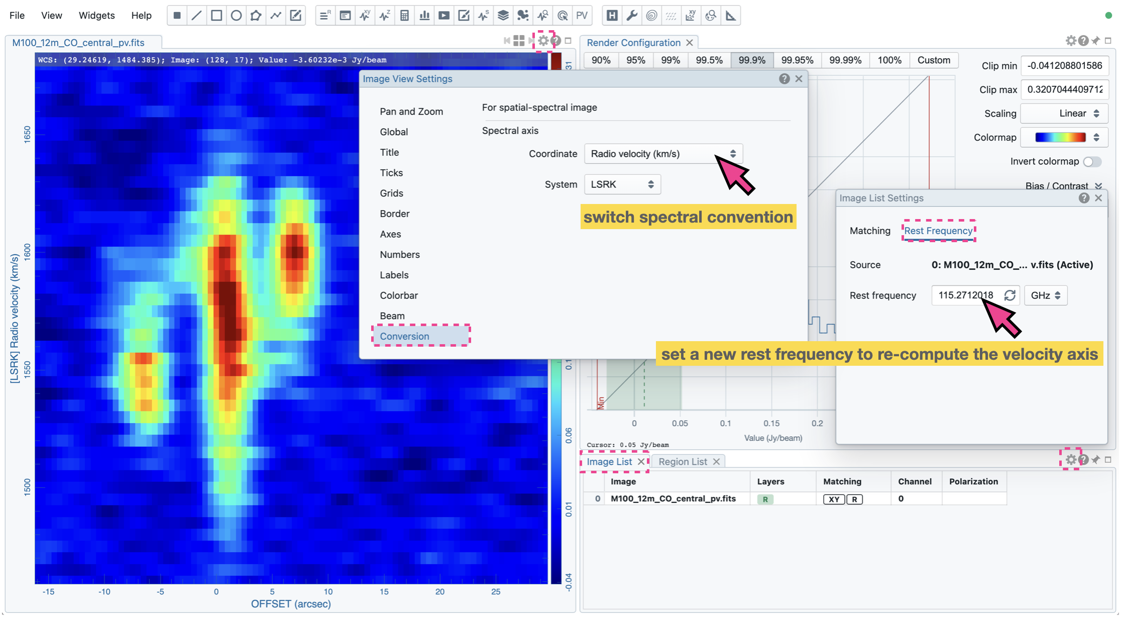
CARTA switches to using rectangular pixels for rendering when a position-velocity image is loaded as a raster image. The pixel aspect ratio is flexible based on the aspect ratio of the Image Viewer Widget. By default, the “spectral” axis is displayed in velocity, if possible, based on the image header. You may use the Image Viewer Settings Dialog to apply a conversion to other spectral conventions, such as frequency or wavelength. The frequency-to-velocity conversion requires a reference rest frequency. This reference rest frequency is derived from the image header. You may use the settings dialog of the Image List Widget to set a new reference rest frequency to recompute the velocity axis.

Contour rendering

In addition to raster rendering, CARTA supports contour rendering as well. A contour image layer can be created on the same raster image or a different raster image with world coordinates matched. The contour generation process is achieved with the Contour Configuration Dialog, which can be launched via the dialog bar.

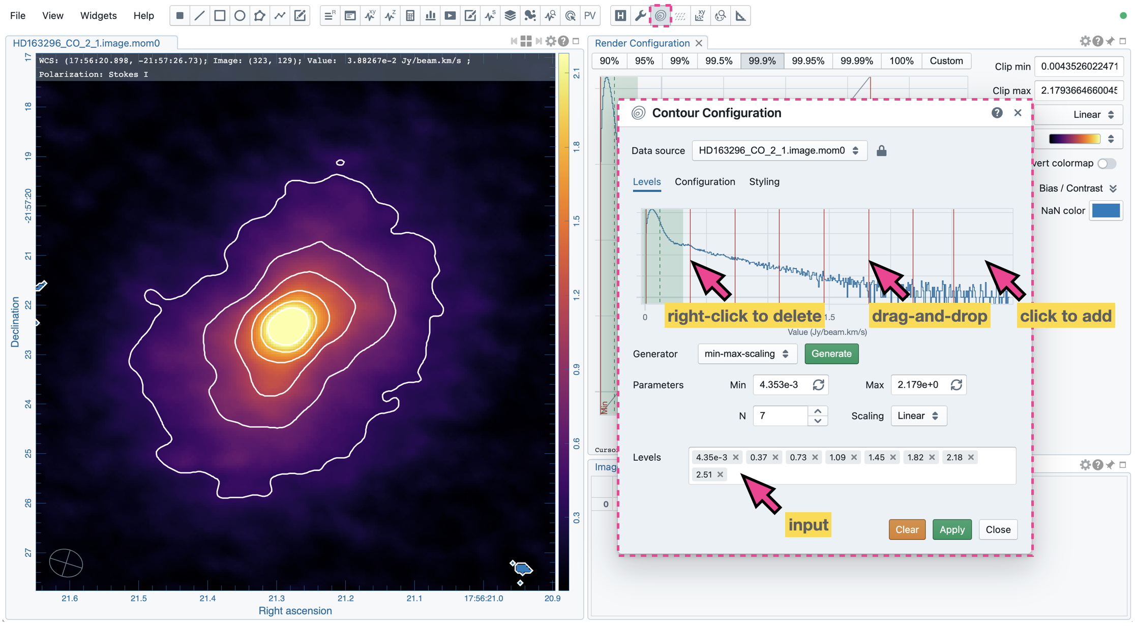
You can follow the steps to generate a contour image:

1. Define contour levels. There are several ways to define a set of contour levels to be calculated on the server side:

1. by typing in individual levels in the “Levels” field manually

2. by using the “Generator” to compute a series of levels

3. by clicking directly on the histogram plot to create levels (right-click on an existing level to remove)

Note that the “Levels” field is editable even if the level generator has generated a set of levels.

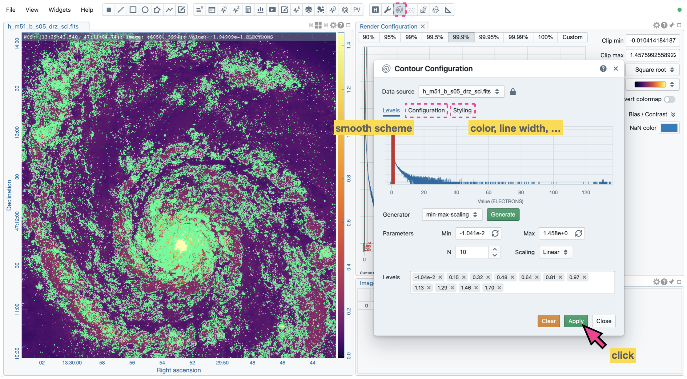
2. (optional) Define a smooth scheme and a kernel size in the “Configuration” tab. The default is Gaussian smooth with a kernel size of 4 by 4 pixels.

3. (optional) Define the appearance of contours to be rendered on the client side in the “Styling” tab. The appearance of contours can be modified after a set of contours has been rendered at the client side without triggering new contour calculations on the server side. This is the advantage of utilizing WebGL2 on the client side.

After defining a set of levels, click the “Apply”” button to view the contour image. The contour image will be rendered incrementally if there are numerous contour vertices.

In the figure above, a contour image is rendered on top of the same raster image. Suppose you want to plot a contour image on top of another raster image (e.g., velocity field as contour, integrated intensity image as raster). In that case, you need to enable WCS matching of the two raster images first (see Matching images spatially and spectrally). Then, you can generate a contour image just like the example below. The contour images will be visible on all the images that are matched to the spatial reference image in world coordinates, including the spatial reference image itself.

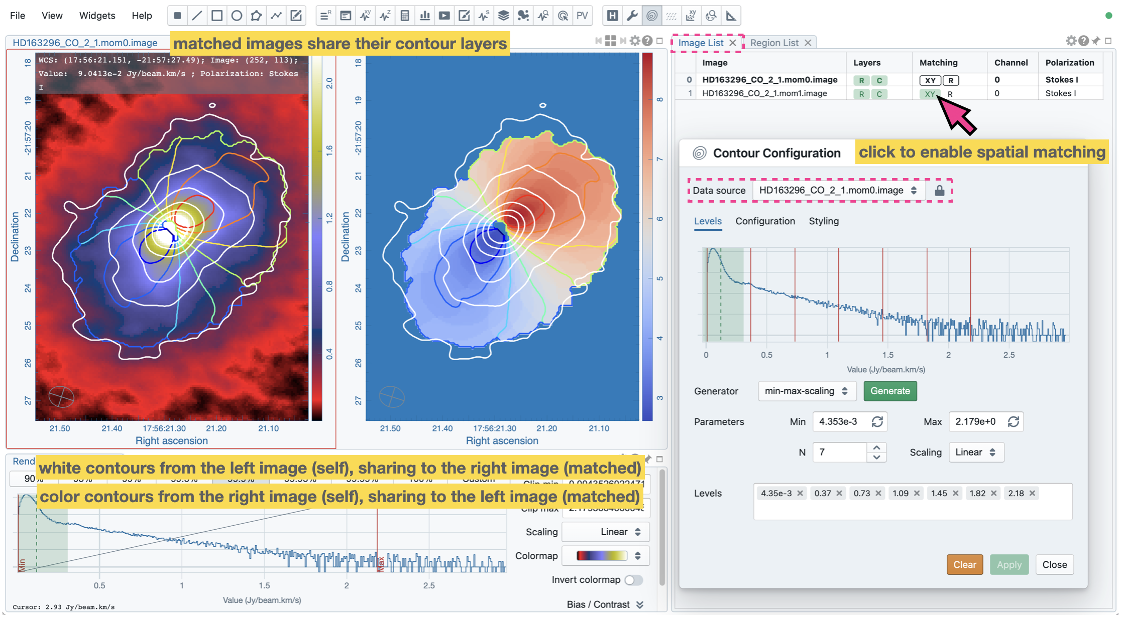
If multiple images are loaded in the append mode, you may use the “Data Source” dropdown menu to select an image as the input data for contour calculations. If the state of the “lock” button is locked, the Image Viewer will show the selected image as a raster image, and the image slider in the Animator Widget will be updated to the selected image too. To turn off this synchronization, click the “lock” button to set the state to unlocked.

CARTA provides four different level generators to assist you in defining a set of contour levels.

• “start-step-multiplier”

  A set of “N” levels will be computed from “Start” with a (variable) “Step” and a “Multiplier”. For example, if start = 1.0, step = 0.1, N = 5, and multiplier = 2, five levels will be generated as “1.0, 1.1, 1.3, 1.7, 2.5”. The function of the multiplier is to make the step increase for each next new level. Default parameters derived from the full image statistics (per-channel) are:

  • start: mean + 5 * standard deviation

  • step: 4 * standard deviation

  • N: 5

  • multiplier: 1

• “min-max-scaling”

  A set of “N” levels will be calculated between “Min” and “Max” based on the “Scaling” function. For example, if min = 2, max = 10, N = 5, scaling = “linear”, five levels will be generated as “2, 4, 6, 8, 10”. Default parameters derived from the full image statistics (per-channel) are:

  • min: lower bound of 99.9% clip

  • max: upper bound of 99.9% clip

  • N: 5

  • scaling: “linear”

• “percentages-ref.value”

  A set of “N” levels will be derived as the percentages (”Lower(%)” and “Upper(%)”) of the “Reference” in linear spacing. For example, if reference = 1.0, N = 5, lower(%) = 20, upper(%) = 100, five levels will be generated as “0.2, 0.4, 0.6, 0.8, 1.0”.

  • reference: upper 99.9% clip

  • N: 5

  • lower(%): 20

  • upper(%): 100

• “mean-sigma-list”

  A set of “N” levels will be generated as “Mean” plus multiples of “Sigma” based on the “Sigma list”. For example, if mean = 1, sigma = 0.1, and sigma list = [-5, 5, 10, 15, 20], five levels will be generated as “0.5, 1.5, 2.0, 2.5, 3.0”. Default parameters derived from the full image statistics (per-channel) are:

  • mean: full image mean value

  • sigma: full image standard deviation

  • sigma list: [-5, 5, 9, 13, 17]

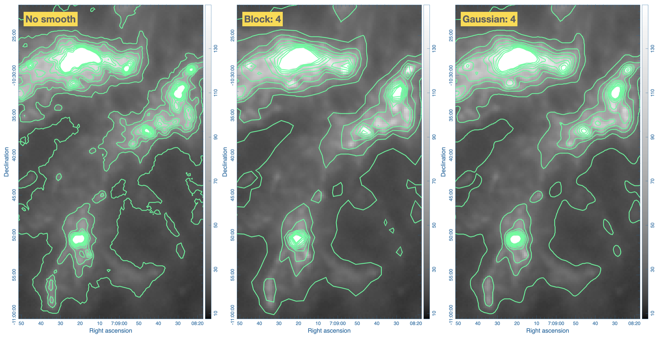
CARTA provides three different contour smoothing methods, including “no smooth”, “Gaussian smooth”, and “block smooth”, in the “Configuration” tab. The kernel for smoothing is in N by N pixels. The default is to apply “Gaussian smooth” with 4 pixels by 4 pixels as the kernel size. You may choose a different smooth method and kernel size depending on science cases.

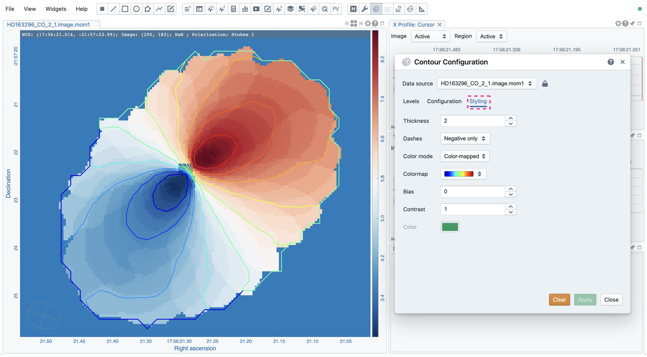
The appearance of contours can be customized in the “Styling” tab. For example, you may use the options to plot contours like below. Iso-velocity contours are rendered in different colors to represent the Doppler shifts of the source kinematics.

Vector field rendering

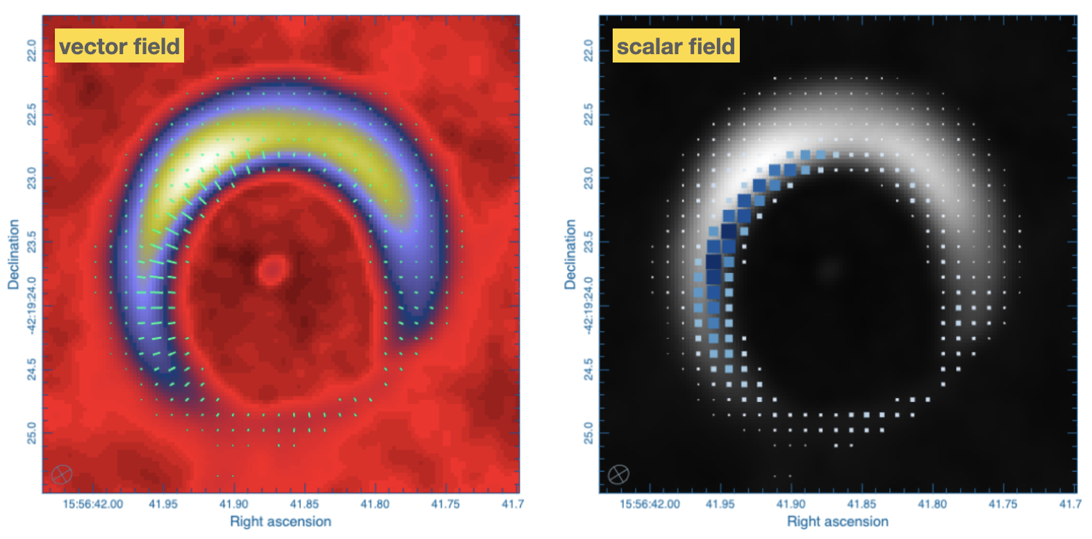
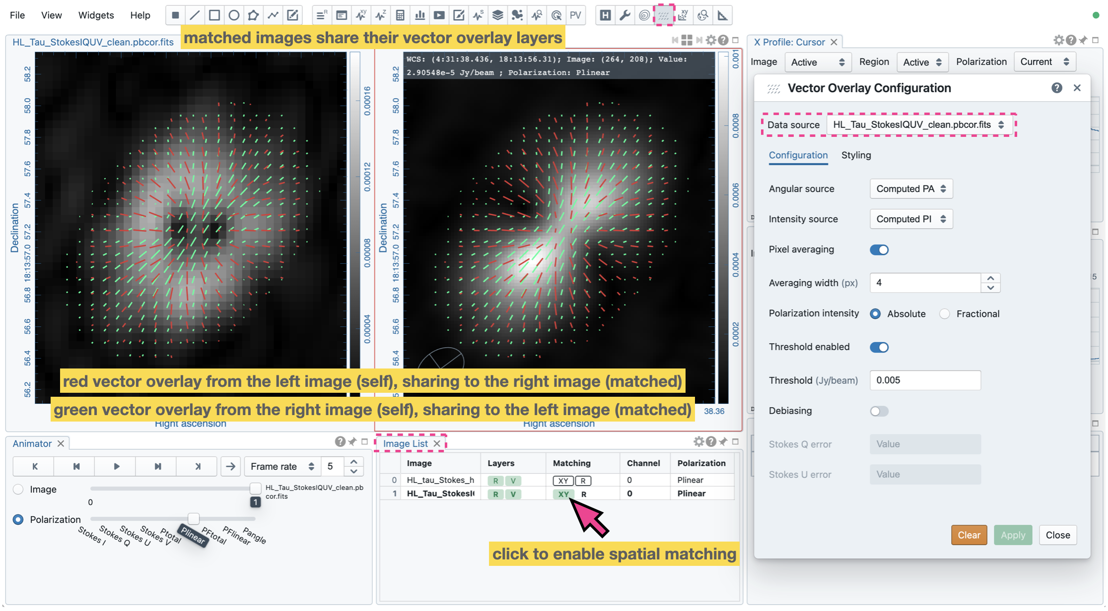
A vector overlay can be added to the Image Viewer from a vector field derived from an image, such as a linear polarization field or a magnetic field, or from a scalar field derived from an image, such as a temperature field or a column density field via the Vector Overlay Configuration Dialog.

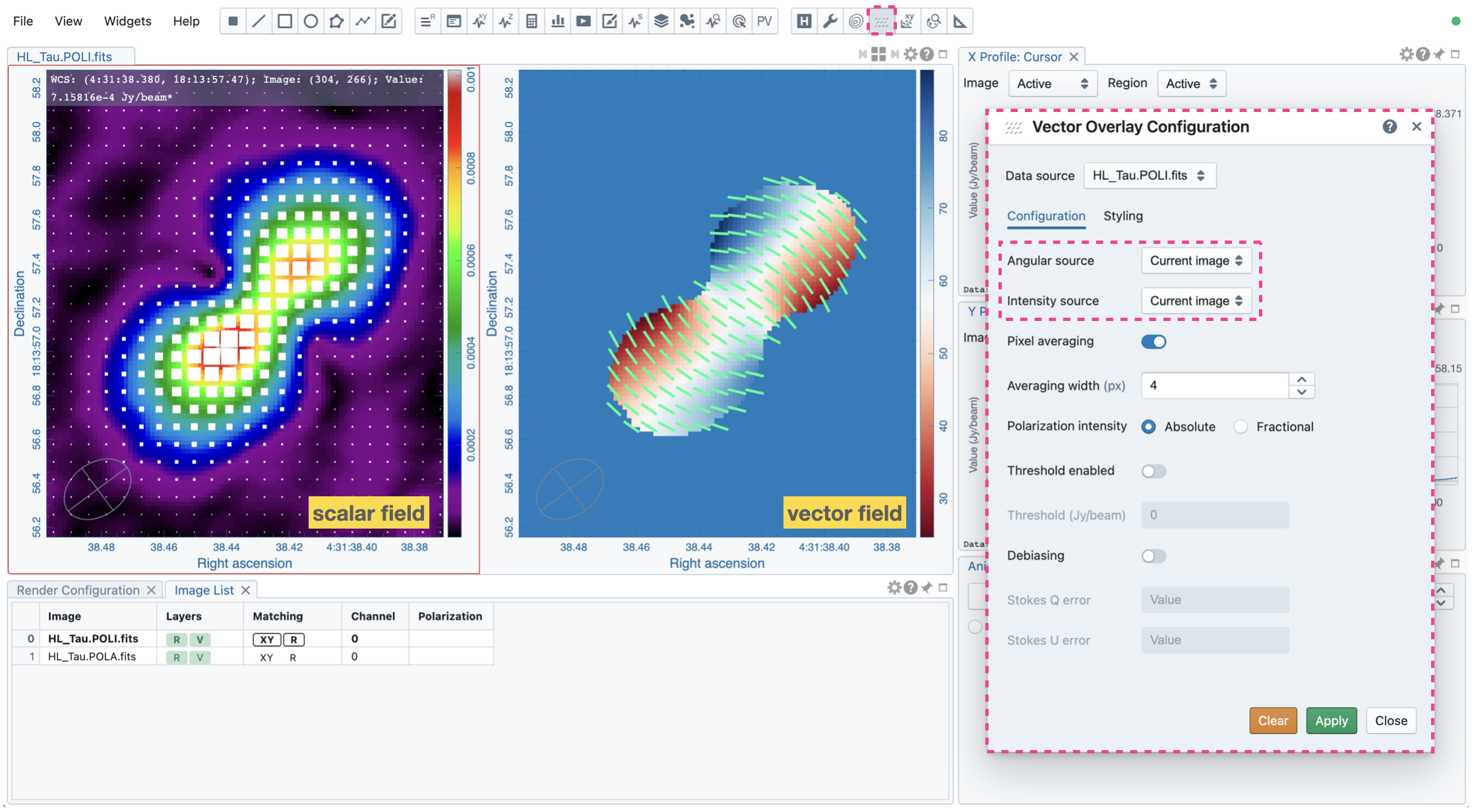
There are different ways to configure how a vector element is derived from the “Data source” via the “Angular source” and the “Intensity source” dropdown menus:

1. For visualization of linear polarization from a Stokes IQU or QU cube with variable vector length and angle, set the “Angular source” to “Computed PA” and set the “Intensity source” to “Computed PI”.

2. For visualization of linear polarization from a Stokes IQU or QU cube with fixed vector length and variable angle, set the “Angular source” to “Computed PA” and set the “Intensity source” to “None”.

3. For visualization of linear polarization from a pre-computed position angle image in degrees, set the “Angular Source” to “Current image” and set the “Intensity source” to “None”.

4. For visualization of a scalar field by interpreting pixel value as the strength or intensity, set the “Angular source” to “None” and set the “Intensity source” to “Current image”. This mode renders a filled square marker instead of a line segment.

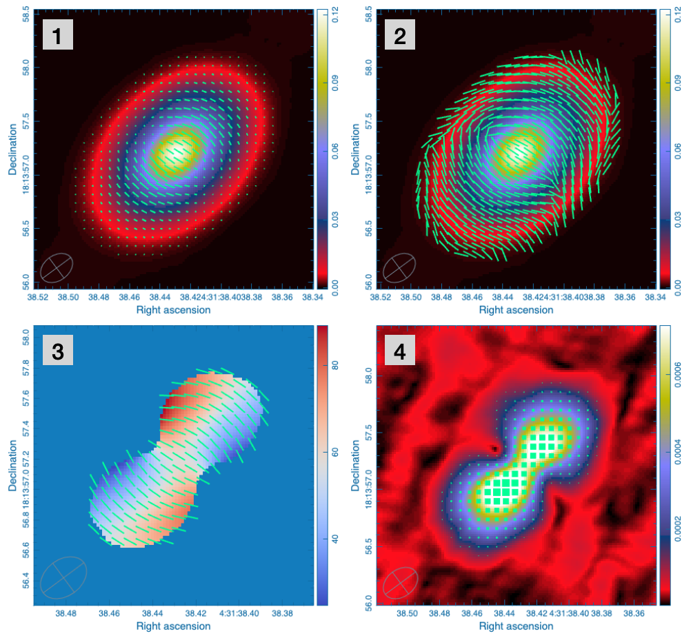
See the figure below for examples of the four vector overlay rendering modes.

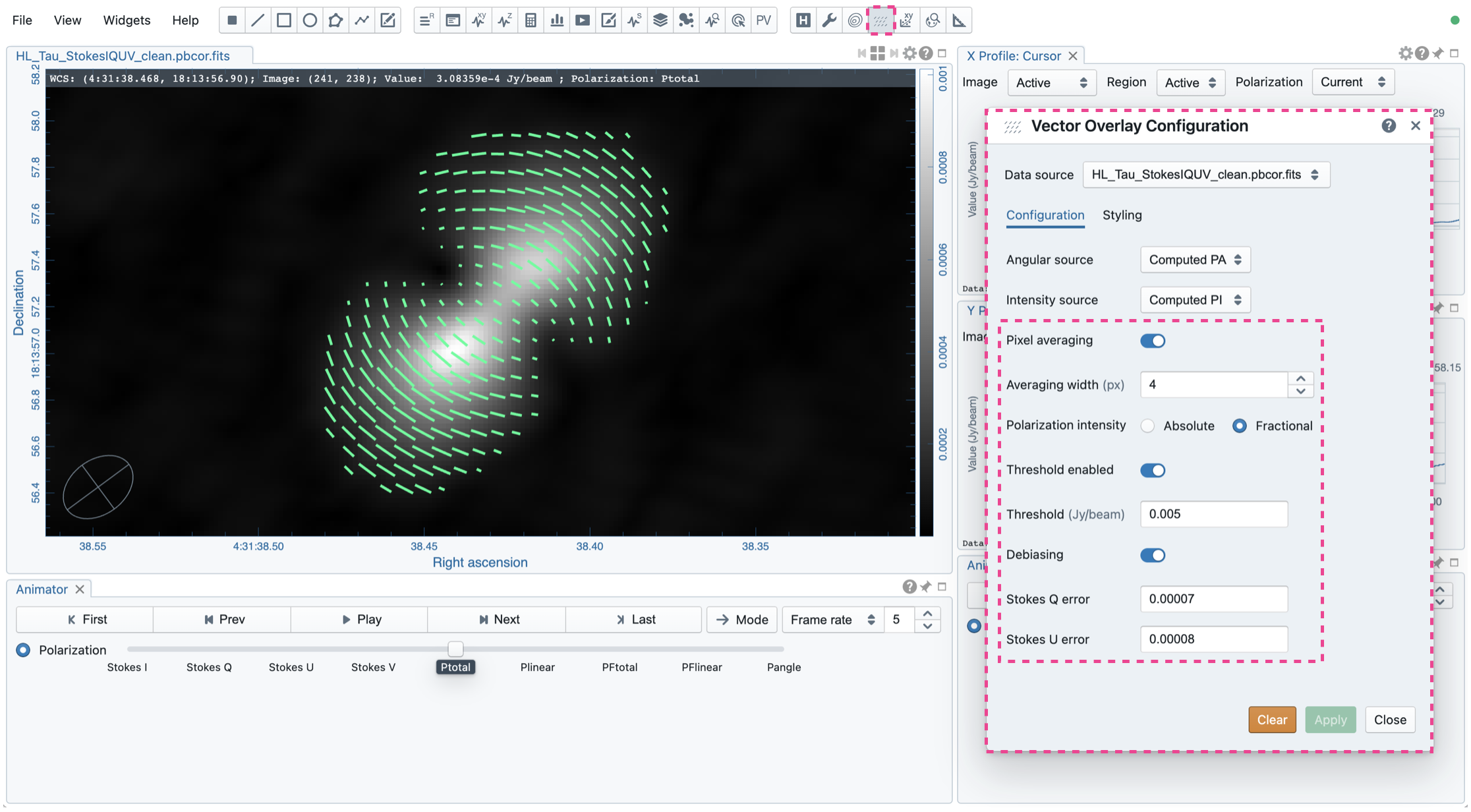
Usually, block smoothing is applied to the “Data source” image to enhance the signal-to-noise ratio before computing vector elements. You can enable the “Pixel averaging” toggle (enabled by default) and set the “Averaging width (px)” (default 4 pixels by 4 pixels) to apply pixel averaging.

When the “Intensity source” is “Computed PI”, you can select “Absolute” or “Fractional” polarization intensity with the “Polarization intensity” radio buttons. A threshold for Stokes I may be applied to mask out noisy parts of the image with the “Threshold” field when the “Threshold enabled” toggle is switched on. If Stokes I is unavailable (i.e., the input image has Stokes Q and U only), the threshold is applied to Stokes Q and U to construct a mask. Optionally, you may apply “debiasing” to the polarization intensity and angle calculations by enabling the “Debiasing” toggle and set errors for Stokes Q and U in the “Stokes Q error” and the “Stokes U error” fields, respectively.

Once the control parameters of how a vector overlay is computed are set, you can click the “Apply” button to trigger the computation and rendering process. The vector overlay data will be streamed incrementally similarly to the raster rendering with image tiles. Click the “Clear” button to remove the vector overlay.

On spatially matched images, vector elements are reprojected precisely based on the projection schemes. This behaves the same as the contour overlay and catalog image overlay. You can use the Image List Widget to trigger image matching.

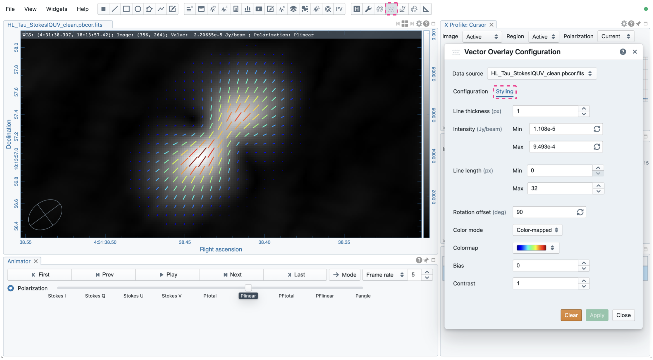
With the “Styling” tab, you can configure how vector elements are rendered, including:

• line thickness

• intensity to vector length mapping

• additional rotation offset to vector angle

• color modes of vector elements

For example, you may use the options to plot a vector overlay like below. Vector elements are rendered in different colors to represent the relative strength of the linear polarization intensity. An angle offset of 90 degrees is applied to the vector elements to infer the magnetic field morphology.

Matching images spatially and spectrally

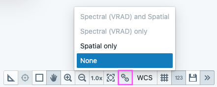
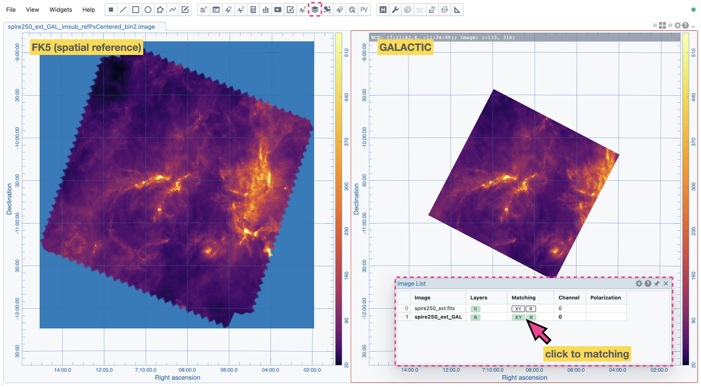
You may trigger image matching based on their world coordinates when multiple images are loaded in CARTA. It is a common practice to compare images from different telescopes or even from the same telescope with different spectral and spatial setups. You can use the “Matching” column of the Image List Widget to trigger the image-matching process,

or the tool button in the Image Viewer.

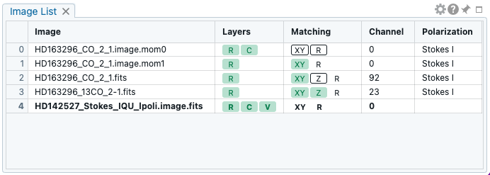
The Image List Widget shows a list of all loaded images, including their:

• file name

• rendering type (“Layers” column): “R” means raster, “C” means contour, and “V” means vector overlay

• image matching state (“Matching” column):

  • “XY” means the spatial domain

  • “Z” means the spectral domain

  • “R” means the color range for raster rendering

• channel index

• polarization component

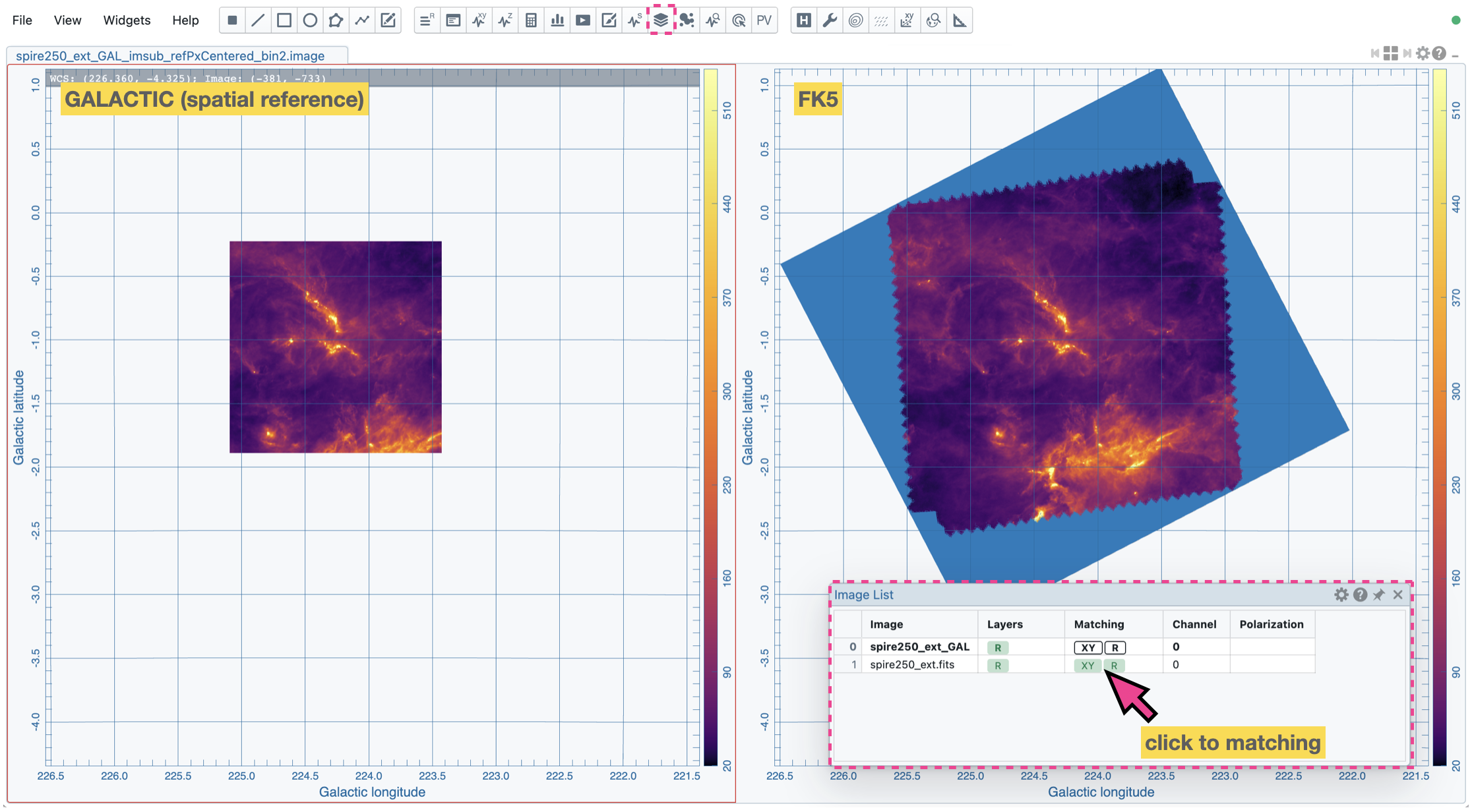
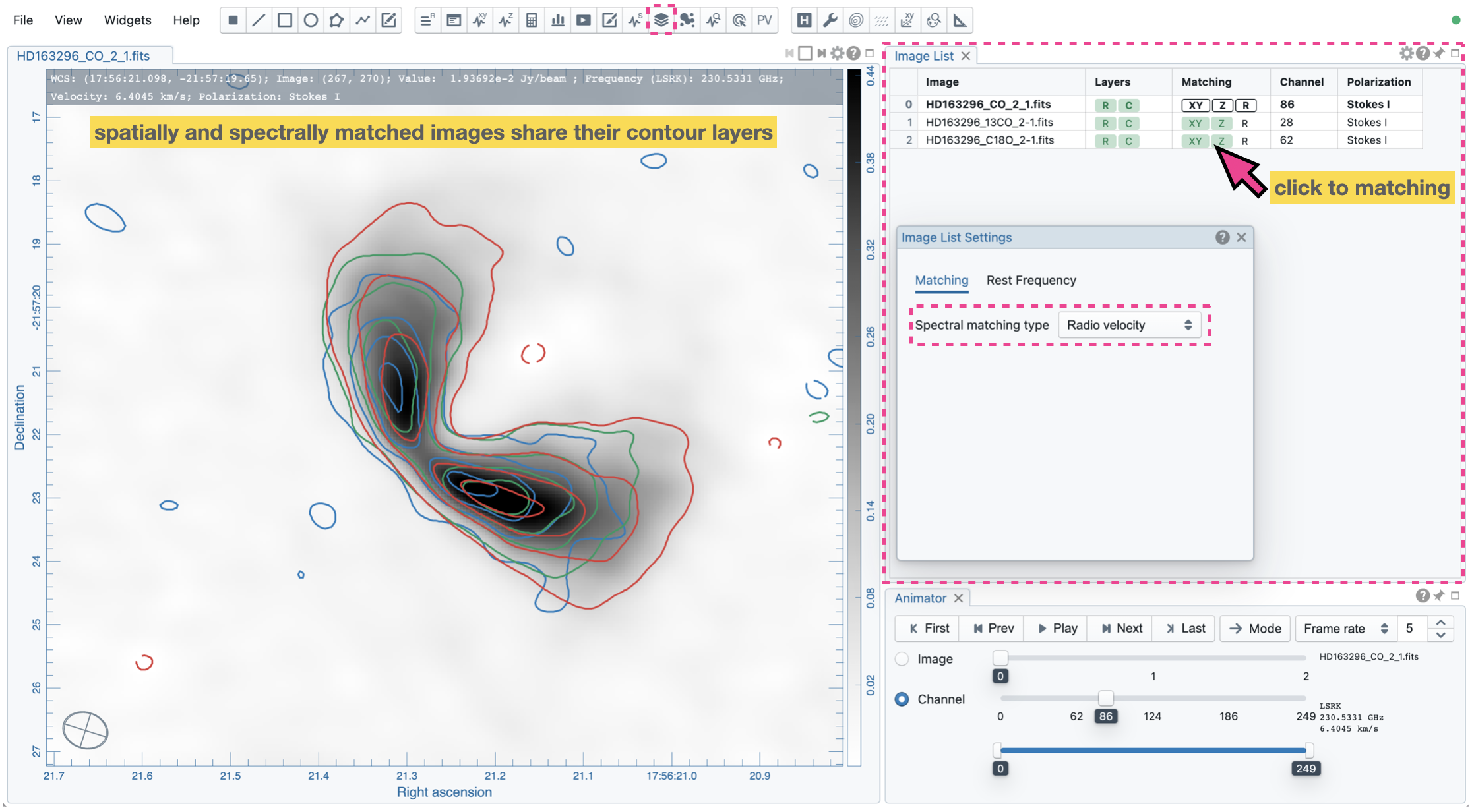
The first loaded image with valid spatial world coordinates serves as the default spatial reference and is highlighted with an open black box (e.g., HD163296_CO_2_1.image.mom0 in the above example). Similarly, the first loaded image with valid spectral coordinates serves as the default spectral reference and is highlighted with an open black box (e.g., HD163296_CO_2_1.fits in the above example). To match the world coordinates of other loaded images, you can click the “XY” button to match the spatial domain and click the “Z” button to match the spectral domain. If you would like to apply the same color range for different raster images, click the “R” button so that matched images will have the same color range as the reference image highlighted with an open black box (e.g., HD163296_CO_2_1.image.mom0 in the above example).

You may change a spatial reference image, a spectral reference image, or a raster scaling reference by right-clicking an image in the Image List Widget and using the context menu.

For raster images, matching in the spatial domain is achieved by applying translation, rotation, and scaling to images with respect to the reference image.

For contour images, matching in the spatial domain is achieved by reprojecting contour vertices to the raster image in the view. Multiple contour images can be displayed on top of a raster image if spatial matching of the target contour image is enabled.

For image cubes, matching in the spectral domain is achieved by nearest interpolation with the target spectral convention. The default is “radio velocity”. The reference convention of spectral matching is configurable with the settings dialog of the Image List Widget. When spectral matching is enabled by clicking the “Z” button, the matched channel indices are updated in the Image List Widget. Images and spectral profiles in the Image Viewer Widget and in the Spectral Profiler Widget are updated, respectively.

Note

Projection effects of raster images

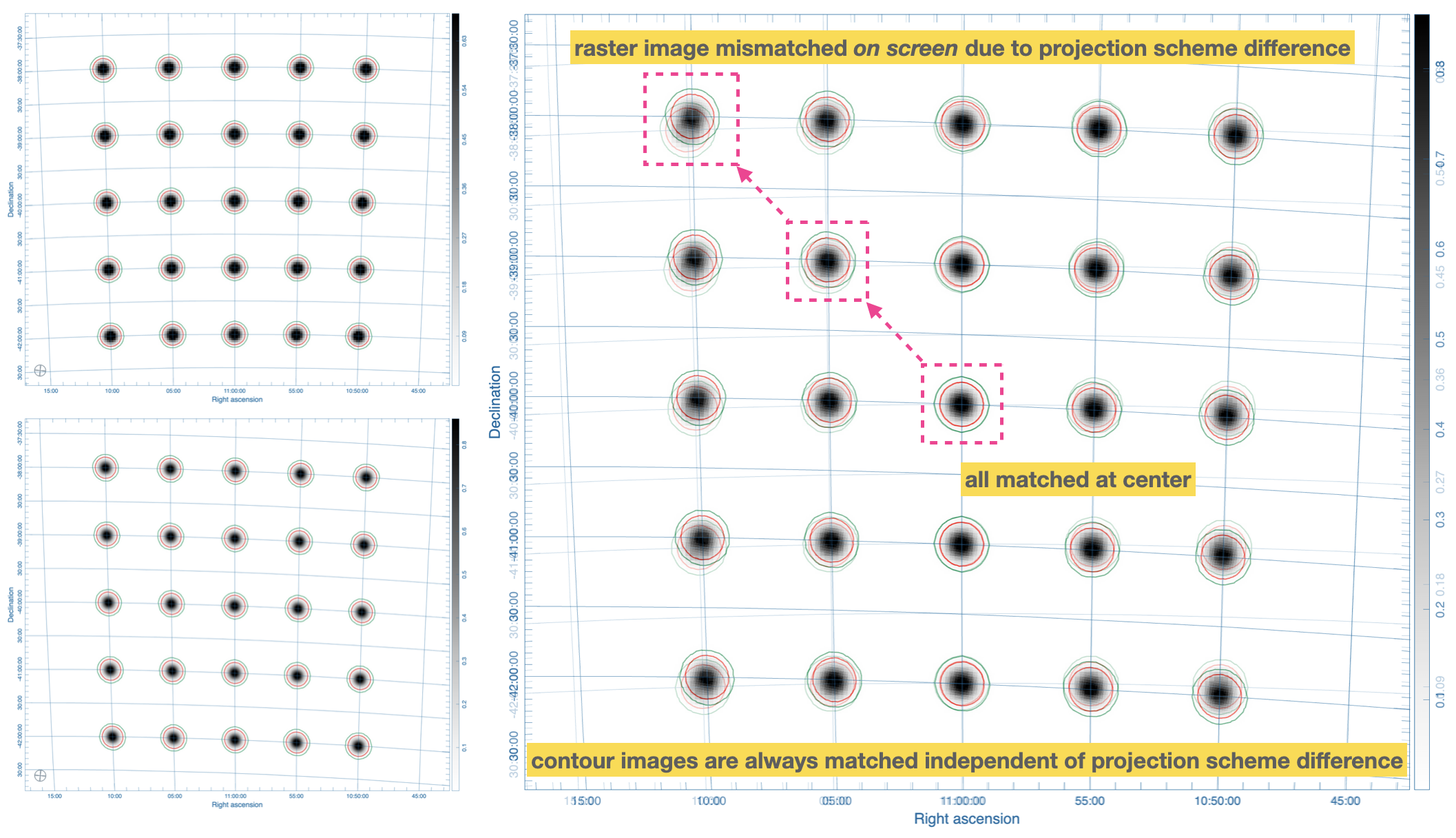
As raster images are matched spatially by applying translation, rotation, and scaling, projection effects between different images might be visible if images have a wide field of view and/or have very different projection schemes. In the following example, projection effects in raster images are demonstrated. However, the projection effects of contour images are properly handled in CARTA. Contours are reprojected with sufficient accuracy to the raster image, as seen in the Image Viewer.

Note

If a spatial reference image or a spectral reference image is closed via the menu “File” -> “Close image”, all matched images will be unmatched, and a new reference image will be automatically registered.

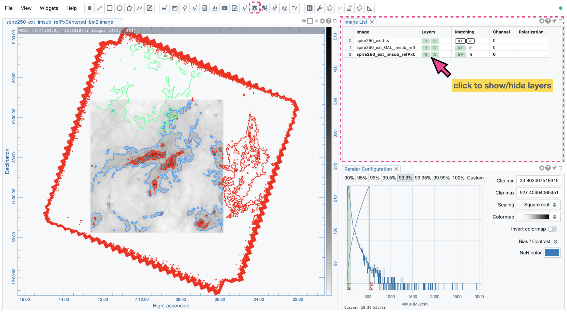
A raster image, contour image, or vector overlay image may be hidden in the Image Viewer by clicking the “R” button, the “C” button, or the “V” button of the “Layers” column in the Image List Widget, respectively. For example, you can create an image with contours only by clicking the “R” button to hide the raster image.

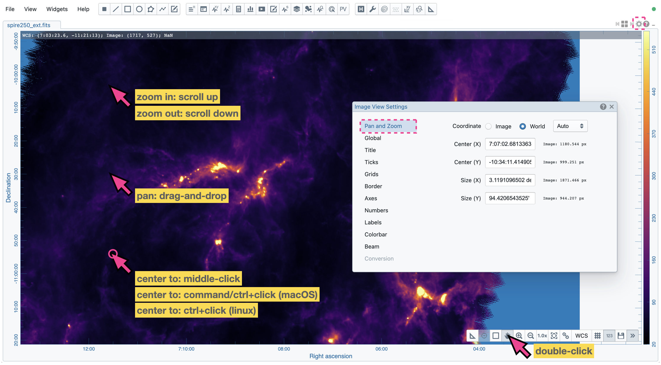
Changing image field of view

You can configure the field of view of the image in the Image Viewer by using mouse actions. If precise control of the position and zoom level of the image is needed, you can use the “Pan and Zoom” tab of the Image Viewer Settings Dialog for the purpose. The same dialog can be enabled by double-clicking the “pan” button in the toolbar of the Image Viewer.

Configuring an image plot for presentation

CARTA provides flexible options to configure the appearance of an image plot. The Image Viewer Settings Dialog is accessible by clicking the “cog” at the top-right corner of the Image Viewer Widget.

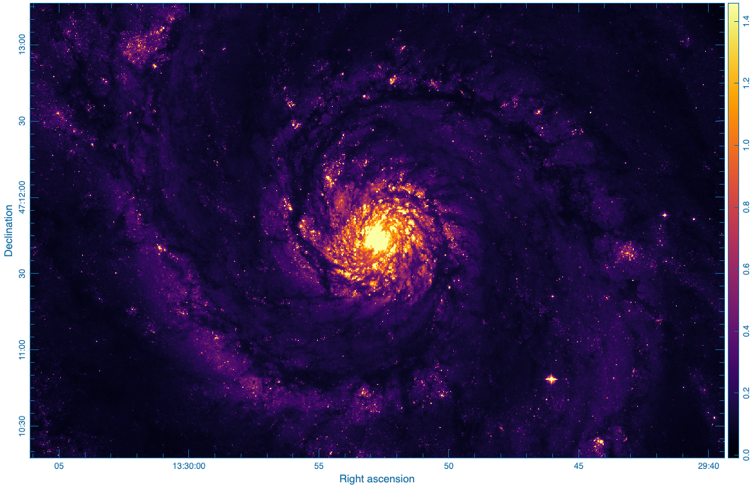
For example, below is an image with default overlay settings.

The image below is a customized one. The coordinate system has been switched from FK5 to GALACTIC. Font type, size, colorbar, axis border and grid lines are customized.

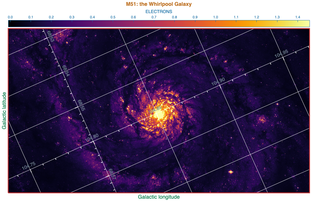
The restoring beam is shown at the bottom-left corner, if applicable.

When multiple images are loaded in the append mode, their loading order determines the order in the image slider of the Animator Widget and the rendering order in the multi-panel view (left-right, then top-down). You can change the order by dragging an entry to a desired place in the Image List Widget.

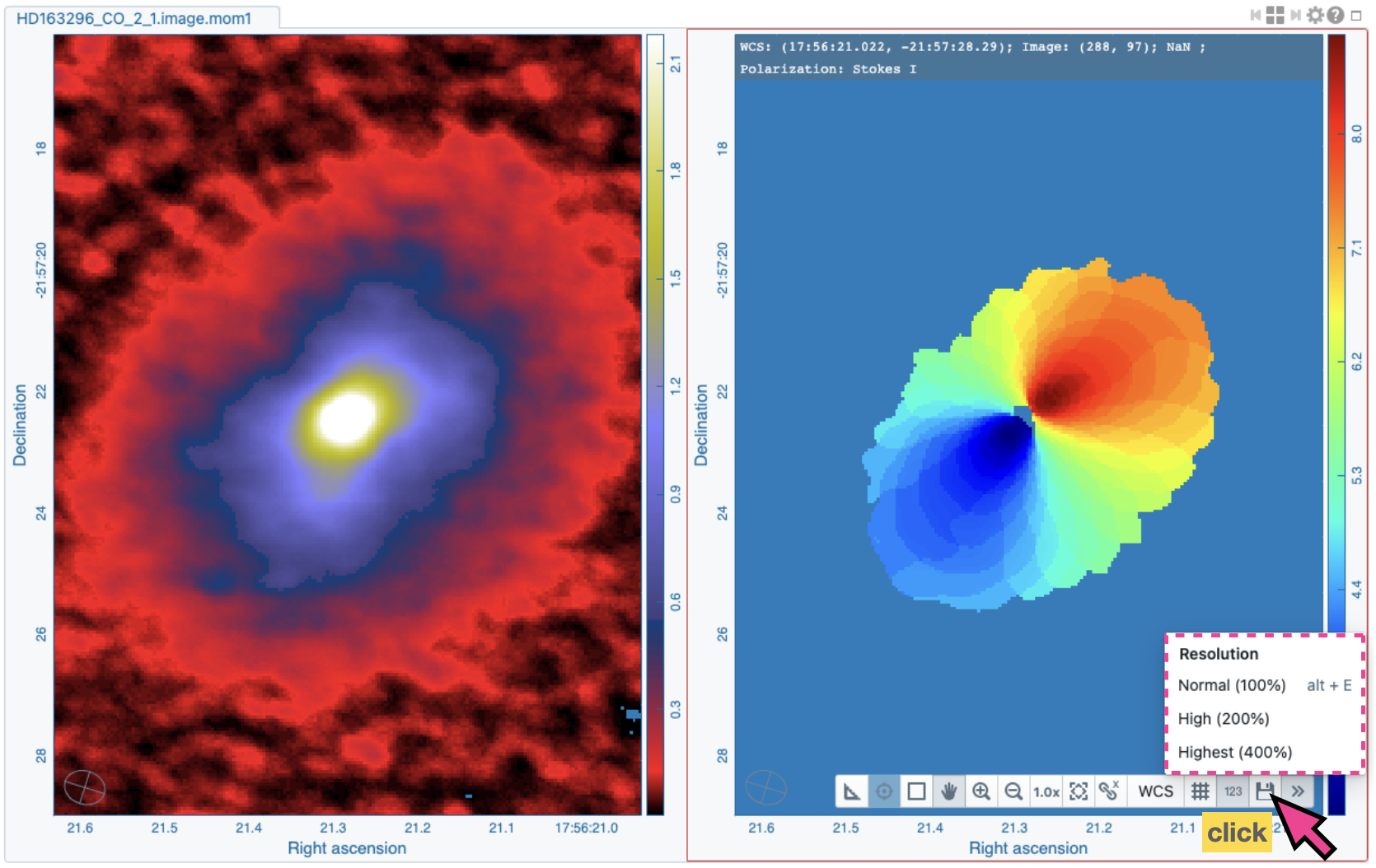
The image can be exported as a PNG image by clicking the “Export image” button at the bottom-right corner of the Image Viewer or by “File” -> “Export image”. High-resolution PNG images can be requested with the additional “200%” and “400%” options. With the “100%” option, the resolution is the same as the screen resolution. With these options, you can set the resolution as 1X, 2X, or 4X the screen resolution. Note that if you use a high-resolution screen to export a PNG image and the request resolution exceeds the limitation of WebGL2, the final resolution of the PNG image will be reduced automatically.

Depending on the theme, a background layer in white or black will be added to the PNG file by default. If you prefer a transparent background, please go to “File” -> “Preferences” -> “Global” and set the “Transparent image background” toggle to false.

Animator

The Animator Widget provides controls for image frames, channels, and polarization. When multiple images are loaded via “File” -> “Append image”, the “Image” slider will show up and allow you to switch to a different image. You can also use the Image List Widget for image switching. If an image file has multiple channels and/or polarization components, the “Channel” and/or the “Polarization” slider will appear. The double slider right below the “Channel” slider allows you to specify a range of channels for animation playback. On the top is a set of animation control buttons such as “Play”, “Next”, etc. Playback modes, including “forward”, “backward”, “Bouncing”, and “Blink”, are supported. Playback action will be applied to the slider with the activated radio button.

The polarization slider shows all the polarization components (Stokes I/Q/U/V, XX/YY/XY/YX, or RR/LL/RL/LR) as defined in the image header. If the Stokes parameters are defined in the image header, additional computed components, including:

• Ptotal: total polarization intensity (computed from Stokes QU or QUV)

• Plinear: linear polarization intensity (computed from Stokes QU)

• PFtotal: fractional total polarization intensity (computed from Stokes IQU or IQUV)

• PFlinear: fractional linear polarization intensity (computed from Stokes IQU)

• Pangle: linear polarization angle (computed from Stokes QU)

are appended as well. You may save a computed component as a new image file via “File” -> “Save image”.

The “Frame Rate” spin box controls the desired frame per second (fps). The actual frame rate depends on image size and internet condition. Optionally, you can set a step for the animation playback (default as unity). By clicking the “Frame Rate” dropdown, the “Step” option will show up.